Implementation of Linear Geographically Weighted Regression

As described in the About GWR page, SpaceStat takes a unified approach to all regression methods, allowing a model to be specified with both geographic and non-geographic weights.  This approach means that as long as an aspatial analysis has been performed on a point dataset (such as a set of polygon centroids), the same model can be run using both aspatial and geographically weighted regression (GWR) methods.  When all points have the same geographic weight, the results for the aspatial and geographically weighted models will be the same.  Thus, our description of the implementation of the various forms of GWR (linear, described on this page, Poisson, and logistic) is very similar to the implementation pages for the aspatial form.  

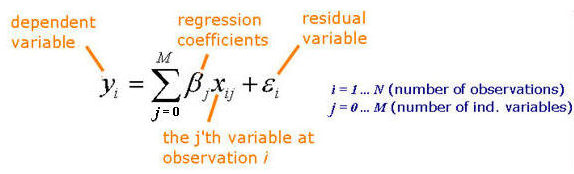
We'll start the description of how linear GWR is implemented with the general equation (below), and then review the approach SpaceStat uses to obtain parameter estimates, sums of squares, R-squared, and p-values.  

Obtaining the local parameter estimates

SpaceStat computes local parameter estimates for linear GWR using a maximum likelihood approach.  Used in this context, "likelihood" refers to the probability that the dependent variable can be predicted from the independent variable(s).  Given the probability function for a single observation, we can write the joint probability function (likelihood function) as a product of the individual probabilities.  In the following equations, the brackets around the beta, which symbolizes the regression coefficients, indicates that we are estimating two or more regression coefficients.

 

Next, we need to define the probability function for the individual observations (on the right side of our equation above), which is shown below.  For linear regression, probability densities are normally distributed (Gaussian), with a zero mean for the residuals and a variance which can differ between observations (note the "i" subscript for the variance components of the equation).  Recall that the symbol (pi), represents a constant (approximately 3.14).  

To estimate parameter values, we use -2 times the logarithm of the Likelihood, because this form has properties that facilitate the likelihood estimation process.  In addition to making this change, we also change how the variance is expressed to allow the incorporation of both geographic and non-geographic weights.  The variance in the equation above can vary by observation; in the equation below, we have replaced the original variance expression with one that includes a constant variance and a weighting factor that varies by observation (see highlighted part of the equation).  Thus, we can now think of the non-constant variance as being equivalent to a weighting factor that varies by observation, times a constant variance.

To solve for the regression coefficients (parameter estimates), SpaceStat finds values for these coefficients that minimize the weighted sum of squares.  The actual computation of the parameter estimates involves operations on a suite of matrices and vectors, and is summarized below.  Note that X with the superscript " T" refers to the transposed X matrix.

Referring back to the regression equation above, the independent variable observation matrix X is regarded as a fixed quantity linking the random error (assumed to have a mean of 0 and a variance ) with the observed values of the dependent variable y, and with the regression coefficients.  Hence, the mean value and standard error of the regression parameters can be obtained in terms of the regression parameters themselves, the inverse of the combination ( XTWX)-1 and the error variance .  The expected value of the dependent variable at each location comes from the product of the independent variable matrix and the vector of the least squares regression coefficients.  These expected values of y are then used to calculate the residual sum of squares and total sum of squares (see below).  

Evaluating the local model:  Calculating sums of squares

As described above, after obtaining the local parameter estimates, SpaceStat calculates the estimated mean, standard error, and residual error for the dependent variable (y) at each observation.  These values are then used to calculate the residual sum of squares (RSS) and the total sum of squares (TSS) using the formulas below.  Recall that "N" is the number of observations, and "M" is the number of independent variables. In the TSS formula, the "y-bar" term represents the mean value of the dependent variable observations.  Recall that these calculations are done repeatedly across the "neighborhoods" in your dataset, and the results can be mapped.  

Local Model R-squared, and R-squared for coefficients

The residual sum of squares and the total sum of squares are used to calculate local model R-squared values, a measure of the strength of the association between the model developed using the geographically weighted independent variables, and the geographically weighted observed values of the dependent variable y.  R-squared values are reported for results using the whole model, and for results for each estimated parameter (regression coefficient) alone.  For aspatial linear regression, SpaceStat also reports an adjusted R-squared value, but this is not available for GWR models.  

Significance of the regression model and the ANOVA table

In contrast to the "global" tool, aspatial regression, GWR does not produce local significance values for the overall model.  In part, this is because the relationship between different independent variables and the dependent variable can vary in different ways across space, and these measures would mask this variation.   Production of local ANOVA tables (described here for aspatial linear regression) would lead to excessive amounts of output in the log view (a table for each point in your dataset).

Local significance of model coefficients

After SpaceStat has calculated the parameter estimates through the Maximum Likelihood estimation procedure, local measures of the individual significance of each can be obtained by using the regression matrix to relate their standard errors to the local model's error variance.  As the regression coefficient values are obtained as sample estimates, a t-distribution with N-M-1 degrees of freedom is used to obtain the coefficient p-values.