Disparity Statistics

As described in the overview, SpaceStat includes two statistics for assessing disparity between different populations in various measures of health, such as cancer rates.  The first is an absolute measure of differences between two rates, and the second is a relative measure, or ratio, which allows assessment of whether disparities between groups are shrinking or expanding relative to changes in mortality rates.  The formulas presented here follow the form and notation of Goovaerts et al. 2007, including the subscript "I" for the absolute measure, and "VI" for the relative measure.  The only difference between SpaceStat' implementation of these techniques and the published version is that, in the absolute measure, Goovaerts et al. (2007) take the absolute value of the numerator.  The formulas here correspond to the "usual" situation of a two-sided test; for one-sided tests of hypotheses, see versions of these statistics that test differences in disparities relative to a threshold value that you specify.

Standardization of disparity comparisons

Note that The Centers for Disease Control and Prevention (CDC) have outlined a method for comparing disparities that attempts to standardize how these comparisons are made, so that analyses can be more easily compared across studies and over time (Keppel et al. 2004).  First, they suggest that disparities should be compared in terms of adverse events (e.g., mortality rates rather than survival rates; to follow the same suggestion with education data, you might compare drop-out rates rather than graduation rates).  This standard is important because you can get very different results if you switch to the opposite form of the data, because one type of rate typically has a much smaller magnitude than the other, so the same absolute difference would be represent a very different proportion of the rate.  Second, they suggest the reference population should be defined as the group with the "best" or most favorable rate (Keppel et al. 2004).   We have followed these guidelines in our implementation of the disparity statistics.  Of course, when looking at a large geography, you may have variation across space and/or time in which of the two populations being compared has lower rates.  To follow the CDC suggestions strictly, we would switch the Target and Reference accordingly in each calculation, but this would hinder our ability to explore space-time patterns in disparity in a meaningful way.  So, we suggest choosing the population that is higher at most locations/times as your Target.    

Absolute Disparity Statistic (Rate Difference)

The absolute disparity statistic for the geographic unit vj is calculated as:

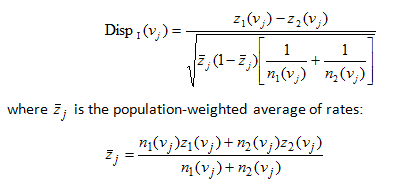
Each rate, z 1(v j) and z 2 (v j ), is computed as the ratio d(v j )/ n(v j ) , where d(v j ) is the number of recorded mortality cases and n(v j ) is the size of the population at risk.

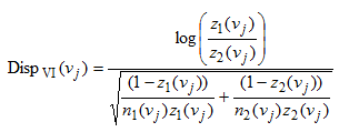
Relative Disparity Statistic (Rate Ratio)

The second disparity measure included in SpaceStat quantifies relative differences between rates measured in different groups.  The formula for this measure is shown below -- note the subscript "VI" has been retained from the original reference.  The variables are defined under the Absolute Disparity Statistic (above).

 

Significance - The Two-sided Test

The significance of the two disparity statistics shown above is assessed using the following procedure, where G(.) is the cumulative probability distribution of the standard normal variable.

 

Corrections for Multiple Tests

When applied to geographic data, evaluations of the significance of test statistics for measures like disparity can easily exceed hundreds of individual tests.  Multiple testing corrections reduce the significance level applied to each test so that the overall false positive rate is kept to less than or equal to the user-specified significance level alpha (typically 0.05, or 1 in 20 comparisons).  Methods to correct for multiple testing differ in their ease of implementation and their stringency. The more stringent or conservative a correction, the fewer false positives are allowed, but this reduction in type I error comes at a cost, in that it leads to a potential high rate of false negatives (type II errors), which in this application would mean that additional observations of disparities would go undetected.  SpaceStat allows you to choose among four options for correction: (1) no correction, (2) the Extended Simes Correction (most conservative), (3) the False Discovery Rate (more powerful), (4) modifying your alpha level.

The Extended Simes Correction

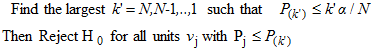
The Simes Correction, described here for applications to local clusters, can be extended across geographies (rather than just across neighbors in the clustering procedures) to account for large numbers of individual tests.  This procedure arose after work by Holm (1979), in which the author proposed an 'improved Bonferroni procedure'; in other words, that procedure that would modify the p-value needed to reject the null hypothesesis that was less stringent than dividing your chosen alpha (typically 0.05) by the number of tests performed (for 10 tests, would then need a P smaller than 0.005 to be considered "significant").  Similar stepwise procedures soon followed, such as the Simes' procedure (Simes 1986) and the 'extended Simes procedure' (Swets 1988).  The approach implented in SpaceStat starts by ranking all p-values from small P(1) to large P(N). The magnitude of the alpha adjustment then decreases as the rank k of the p-value increases, i.e. the division factor applied to alpha is (N-k+1).  

The False Discovery Rate

Instead of controlling type 1 errors (rate of false positives), the False Discovery Rate controls the expected proportion of true null hypotheses rejected out of the total number of rejections.  FDR approaches are thus less restrictive and more powerful than family-wise alpha-protecting tools like the Bonferroni procedure and the Extended Simes Correction.  In SpaceStat, we have implemented an approach developed by Benjamini and Hochberg (1995).  These authors proposed a stepwise FDR procedure for independent tests in which the first step is to rank all p-values by ascending order and apply a correction that decreases as the rank k of the p-value increases, i.e. the division factor is k/N.  Unlike the Extended Simes, the decision rule is sequential, and involves checking that the p-value of rank k does not exceed the adjusted significance level, starting with the larger p-value (k=N).  Once this condition has been met for a given rank k', the adjusted significance level is set to and applied to all tests of hypothesis. The decision rule can then be formulated as:

 

Rate Multipliers and Zero Populations in Disparity Analyses

In many datasets, such as those available from NIH (e.g., the National Atlas of Cancer Mortality), the rate includes a multiplier, such as 100,000.  For this reason, when you go through the steps of calculating disparity statistics, a box at the bottom of the Input page provides a place for you to identify the "Disease Rate Multiplier," and one of the calculation steps will be applying the multiplier to the rate in the selected dataset to obtain a count of occurrences (e.g., cancer mortalities) that can then be divided by the population size.  

If one of the two populations at risk is zero, the disparity statistic is not computed and SpaceStat generates a missing value for that region.

Click here to see information about 1-sided tests (exceedance of thresholds in disparity).

Click here to see how to run a disparity analysis.