Aspatial Linear Regression Output
Here, we will show the output from the model we used to illustrate running a regression model on the "Perform" page. The only change we have made from the previous description is that we have added the word "Linear" to the model title and to the name of the output folder to help us differentiate them from models and output using the other two model types.
Summary of the model run
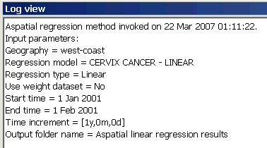
After clicking to the run method page and then selecting "Run", we see the following output in the log view, beginning with the summary of the model run.

Fit and significance of the model as a whole
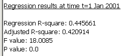
Below the review of the model run information, SpaceStat presents the summary of the predictive ability and significance of the model as a whole for the first time period. The dataset described here only includes one time period, but if you analyzed a set with several time periods, you would see several sets of output, separated by date.

Specifically, SpaceStat lists the model R-squared and adjusted R-squared values, which are measures of the strength of the model's predictive ability. Recall from the "perform" page that if you have chosen to fix your intercept at (0,0), SpaceStat will report the R2 for your "no intercept" model as "-". These R-squared measures, and the method used to calculate the significance of the full model, are described under Model R-squared, and Significance, respectively, on the Implementation of Linear Regression page. Note that significance values in regression output are reported as "0.0" if they are smaller than 0.000001 (see the "P value", above). Thus, the results shown here indicate that our model does a respectable job of predicting cervix cancer risk, with an R-square of 0.44. The model is also highly significant, with a p-value less than 0.000001.
The ANOVA table
The next item in the output is the Analysis of Variance, or ANOVA table, which allows us to evaluate the importance of each individual term in building up the regression model. This first column of this table ("Source") lists all of the terms included in your model - recall this model of cervix cancer risk included three linear terms, the percent of the population that is Hispanic, the percent of the population that does not have health insurance (Noins), the ratio of the general population to the number of doctors (MDratio, categorical). and the interaction between "HISPANIC" and "Noins."

The next column, labeled "D.F." presents the degrees of freedom associated with each term. This value is one for each continuous variable, and for interactions between two or more continuous variables. For categorical variables, the degrees of freedom equals the number of categories minus one (our levels for "MD_Ratio" are high, medium, and low). The degrees of freedom for an interaction term is calculated by multiplying the degrees of freedom from each component. The next two columns, Type III SS (sum of squares) and Mean Square, are used to determine an F-value, which is compared to an F-distribution to calculate the p-value (last column); this is described in more detail on the implementation page. This p-value represents the probability of obtaining an F-value as extreme as the test statistic by chance alone, under the null hypothesis of no effect of the term on the dependent variable (cervix cancer risk). In this example, the first two linear terms are significant (in reference to an alpha of 0.05), but the MDratio term is not, and the interaction term is just above the 0.05 cut-off, with a p-value of 0.065.
Significance of individual model parameters
The next table in the output for aspatial linear regression provides the parameter estimates, standard errors, and p-values for each parameter in the model. See the implementation page for a description of how the p-values are derived. Note that as described on the categorical variables in regression analyses page, a parameter is estimated for each level of a categorical variable, except for the level that is chosen as the reference value (we chose "medium").

Looking at the p-values, we see that in addition to the significant terms identified from the ANOVA table, the model intercept is also significant. For the continuous variables, the p-values are the same as in the ANOVA table, but individual parameter estimates and p-values are shown for the two non-reference values for the categorical variable, MD_Ratio_CAT.
Table of correlation coefficients
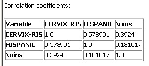
Finally, the last table produced as part of the output for aspatial linear regression shows the correlation coefficient for each pair of numeric variables in your model. This is helpful for understanding how different independent variables are related, and can be used to identify terms that could be dropped from the model due to high correlation with other terms (colinearity).

In this example, all of the correlations between the pairs of continuous independent variables is low, 0.18. Recall that CERVIX-RIS is the name of our dependent variable, smoothed cervix cancer risk.
Note that these values may differ from correlation coefficients presented in the graph statistics window due to the effect of missing values. In the case of the regression model, the correlation will not include data from ANY of the variables at observations where one or more value is missing, while only missing values in the two datasets being compared will influence the correlation coefficient in the graph statistics window in a scatter plot.


