Perform Stepwise Aspatial Regression

The process for performing a stepwise aspatial regression analysis is identical to that described on the "Perform Aspatial Regression" page, except that if you choose forward or backward stepwise regression, you will activate a few additional sections of the regression settings page.  To minimize switching back and forth between Help pages, we repeat those methods here with a different example.  To begin, select Aspatial regression methods by pulling down the Methods menu and choosing Regression -> Aspatial regression.  As with the "full model" version of aspatial regression, you will choose among the various types of regression (linear, Poisson, and logistic) within the regression settings page of the Task Manager.  

In this example, we are working with lung cancer rates for white males (RWM_LUNG) aggregated at the county level for states in the eastern U.S., averaged for the years 1970-1994.   We will demonstrate creating and running stepwise regression models with a suite of seven independent variables that were freely available and provide a useful example (but are not ideal for actual evaluation of patterns, as they correspond to different dates).  Five of these come from the Center for Disease Control and Prevention's Behavioral Risk Factor Surveillance System Survey (CDC BRFSSS, 2004) -- per capita income (PCINCOME), percent of the population over 65 (PEROVER65), percent of the male population that ever smoked (SMOKEVRM), and percent of the population that is obese (OBESE).  In addition, we have radon risk data (three categories) from the EPA's Radon Program, as well as the log of concentrations of xylenes (LOGXYLENES) and tetrachlororethylene (LOGTETRACHLOR) from the EPA's 1997 National Emission Inventory.   We put these data together in a model to simulate steps you might go through when exploring potentially interesting patterns in male lung cancer, and have assigned them all to a time of 1994 so that they can be combined in the same analysis.

One step that we strongly suggest if you have lots of potential variables that may be highly correlated is to first put all of the potential variables you would like to explore in a model (following the directions here or on the "Perform Aspatial Regression" page) and then run a "full model".  This will provide you with a correlation matrix for all of the variables so that you can see which are highly correlated, and then avoid building models with variables that appear redundant.  This step is important because the presence of colinearity can lead to poor estimation of coefficients, and is especially likely when you explore large numbers of potential predictors using stepwise and best subset model building methods.  

Creating and managing regression models

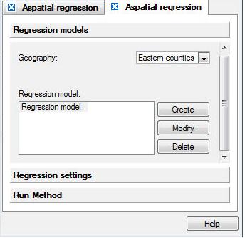
When the task manager opens for Aspatial regression, it will start on the "Regression models" section.  Here, you must choose your geography (if your project contains more than one), and then indicate whether you would like to create, modify, or delete a regression model.  You can create a suite of models that all share the same geography, dependent variable, and form (linear, Poisson, or logistic) within one Aspatial regression "tab" in the task manager, and these will all appear with the default name "Regression model" on this page, unless you change the name (see below).  To modify an existing model, highlight it, and then hit the "Modify" button.  Similarly, select a model and then click on delete to remove it from the list.  Additional models can be created and saved, and they will all be listed in this window.  Note that if you choose the regression method again from the methods pull down window, a new regression tab will appear, and will list the same suite of models (note the two tabs shown below).  You can delete this extra tab without losing your saved models.

Defining a new regression model

When you click on the "Create" button in the initial task manager page for Aspatial regression, a dialog will open where you define the dependent and independent variables that will be included in your regression model.  You can also use the instructions below to modify a model you have already created.

Click on the boxes below for brief definitions, and for links to detailed information on defining the terms in your model.

   

Selecting model terms.

The window titled "Independent variables" lists all of the datasets associated with the geography that you selected in the first Task Manager window for regression.  To use one or more of these datasets as a term in your model, click on it to select it.  To select more than one dataset (for adding an interaction term), hold down the "Ctrl" button as you click on each.  When the dataset name is selected, you can then use the buttons on the right to add that dataset as a linear term (i.e., as an "x"), as a squared term (i.e., as an x2), or as part of an interaction term in which it will be multiplied by one or more other independent variables.  In the example above, we have selected the eight variables described above as linear terms.  As you add various terms, they will appear in the three boxes in the center of the task manager window.  You can delete terms that you have created by selecting them and then using the delete button on your keyboard.

Categorical variables:  Select the reference value and parameterization type.

Directly below the windows where the regression model terms are listed is a section that only applies to categorical variables; in this area you will choose a reference value and a parameterization type (coding system).  These options are explained in detail in the help section on categorical data in regression.  To fill in these options for your categorical variables, first select the categorical dataset ("RADON_CAT" in the example above --note that even though this looks like an integer variable, it is coded as alphanumeric/string).  When a categorical dataset is selected, you will be able to scroll through the names of the categories within that set in the box to the left of "Reference value for...".  Next, for that same categorical dataset, you choose a reference cell or effect cell approach to coding by clicking on the respective circle to the left of your choice.  If you have more than one categorical term, including interaction terms that incorporate a categorical dataset, you will need to repeat this process for all of these terms.  If you forget to do this step, SpaceStat will run the model using the default settings of reference cell parameterization, with the middle category (alphabetically) or last category (for numbers coded as strings) as the reference value.

Fix intercept at zero check box.

Check this box if you want to force your linear regression model through the origin (0,0).  This option should not be applied to Poisson or logistic regression, or to linear regression with only categorical terms.  If you do check the box with a Poisson or logistic model, or for a model with categorical terms, SpaceStat will proceed as if the box had not been checked.  Note that if you have chosen to fix your intercept at zero, SpaceStat will report the R2 for this "no intercept" model as "-".  This is because calculations of R2 in the no-intercept models tend to be larger than models with an intercept, or in some cases can be negative.  Details on this topic are presented in Kutner et al. 2004.

After you have finished creating or modifying your regression model, click "ok" to return to the first page of the task manager for regression, and then click on the "Regression settings" tab to complete the process of defining your model.  

Regression settings.

After you have identified the datasets to be used in your model, you will need to define other settings, including the regression type (linear, Poisson, or logistic), the type of model selection tool you want to use, any weight sets you would like to use, and the time settings.  When you have completed this page, click on the last section, "Run Method".

Click on boxes within the image below for more information.

Run Method

When you click on "Run Method", the Task manager will present a summary of the model you have just created or modified.  If you agree with the model definition that appears in this window, then click on the "Run" button at the bottom of the window to run the model.  Note that the information shown here will be repeated in the log at the beginning of your stepwise regression output.

Now that you have run the model, look in the log view to see your results.  There are some variations in the output presented for the various model types, and it may be helpful to first review the typical output for a "Full model" run of a linear, Poisson, or logistic model before trying to understand the output from stepwise regression.

To see the output for this model run with forward stepwise, click here; for backward stepwise results, click here.