


About Linear Geographically Weighted Regression
Geographically weighted linear regression can be thought of as the local version of aspatial linear regression: Instead of just one global regression equation for the entire dataset, this technique generates parameter estimates for each neighborhood within your spatial dataset. Calculation of local relationships requires choice of a spatial weighting factor, a value that determines how strongly values measured at nearby locations influence the regression equation calculation, and your definition of neighborhood, which will define how many other points are used to estimate the local regression lines. In aspatial regression the weighting factor is set to one for all values in the dataset, and the neighborhood is extended to the entire geography, so values from all locations contribute equally to the regression equation.
In linear GWR, statistical models are fit to sets of N observations (defined by your choice of neighborhood) such that a dependent variable y can be expressed in terms of one or more independent variables, and a residual, or error, term. Independent variables can be continuous and/or categorical, and you can also include squared terms, interaction effects, and weights in your model. Note however that some combinations of categorical variables lead to overspecified models, so read that page to learn about common pitfalls to avoid when defining your model.
The figure below shows a dataset of N=23 points, plotted so that y, the variable we would like to be able to predict, is shown on the vertical axis, and a single independent variable (x) is shown on the horizontal axis. The goal of the linear regression modeling exercise (at a local or global scale) is to find the linear function that provides the best prediction of y; that is, it produces the smallest errors, measured as the squared difference between the observed value of y, and the value of y from the regression line at the same value of x. Note that the term "linear" refers to the linear combination of parameters in the model, and that the graph that results from a linear regression model does not have to be a straight line.

A general equation for linear regression
As in the description of aspatial linear regression, to describe linear GWR we start with the general equation for a linear regression model. In this model, the independent variable observations are regarded as fixed, and all other variables (y, and the error term) are considered random. One way of expressing a linear regression model with an unspecified number of independent variables is shown below. You may be familiar with formulas that separate out a b 0 (y-intercept) term from the rest of the regression parameters, such as the equation for the simple linear regression line that appears here in the SpaceStat help. This parameter is still included in the formula below, in that the "x" part of the "b j x ij" component drops out when j=0.
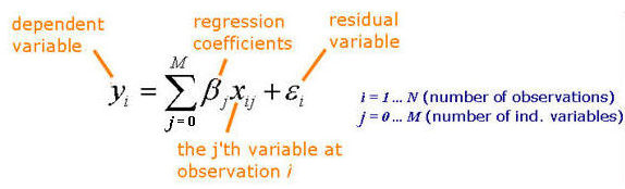
Output from linear regression
SpaceStat output from linear GWR includes R-squared (and adjusted R-squared) values, which measure the fit of the model as a whole, and significance values (p-values) for the whole model, and for individual terms in the model. The output is described in more detail here, including examples from the SpaceStat log view.
To find out more about how linear GWR is implemented in SpaceStat, click here.
To skip the details and learn about how to perform linear GWR, click here.