Perform Geographically Weighted Regression

Geographically weighted regression methods are located under Methods -> Regression -> Geographically weighted regression.  You choose among the various types of GWR (linear, Poisson, and logistic) within the regression settings page of the Task Manager.  

As a general practice, we suggest running all new models with the aspatial regression method first, as some efforts to identify model coefficients using the Maximum Likelihood approach will fail to coverge (see here for more information).  Failure to converge is most likely when using logistic regression, and if a model won't converge in an aspatial form, it will also probably not converge in GWR, and will take much longer to run before failing.

In this example, we are working with a set of breast cancer mortality rates for white females aggregated at the county level for states in the northeastern U.S.  We will demonstrate creating and running a regression model with two linear independent variables: the number of physicians per 1000 patients (MDRATIO), and the log of xylene (a group of benzene derivatives found in petroleum) releases in tons/year, which has been log transformed.  To illustrate the use of an interaction term, our model also includes the interaction between the percent of county residents living below poverty level, and the median age of residents in the county.  The county data began as a polygon geography, but were converted to a centroid coverage for these analyses.

Creating and managing regression models

When the task manager opens for GWR, it will start on the "Regression models" section.  Here, you must choose your geography (if your project contains more than one point coverage), and then indicate whether you would like to create, modify, or delete a regression model.  You can create a suite of models that all share the same geography, dependent variable, and form (linear, Poisson, and logistic) within one Geographically weighted regression "tab" in the task manager, and these will all appear with the default name "Regression model" on this page, unless you change the name (see below).  Note that any aspatial regression models that you have created using a point geography will also appear in this window.  To modify an existing model, highlight it, and then hit the "Modify" button.  Similarly, select a model and then click on delete to remove it from the list.  Additional models can be created and saved, and they will all be listed in this window.  Note that if you choose the regression method again from the methods pull down window, a new regression tab will appear, and will list the same suite of models (an example of this is shown here, for aspatial regression).  You can delete this extra tab without losing your saved models.

Defining a new regression model

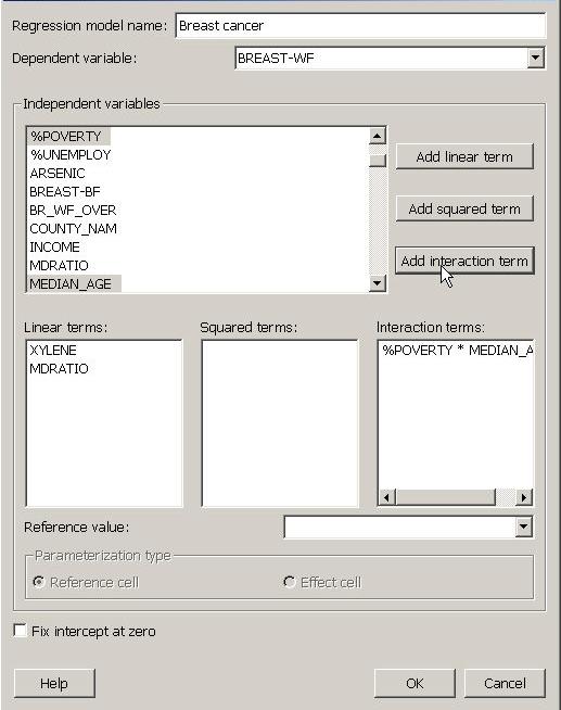
When you click on the "Create" button in the initial task manager page for Geographically weighted regression, a dialog will open where you name your model, and then define the dependent and independent variables that the model will include.  You can also use the instructions below to modify a model you have already created.

Click on the boxes below for brief definitions, and for links to detailed information on defining the terms in your model.

Selecting model terms.

The window titled "Independent variables" lists all of the datasets associated with the geography that you selected in the first task manager window for regression.  To use one or more of these datasets as a term in your model, click on it to select it.  To select more than one dataset (as shown in the image above, for adding an interaction term), hold down the "Ctrl" button as you click on each.  When the dataset name is selected, you can then use the buttons on the right to add that dataset as a linear term (i.e., as an "x"), as a squared term (i.e., as an x2), or as part of an interaction term in which it will be multiplied by one or more other independent variables.  In the example above, we have selected the two linear terms (XYLENE, and MDRATIO), and included an interaction term (%POVERTY * MEDIAN_AGE).  As you add various terms, they will appear in the three boxes in the center of the task manager window.  You can delete terms that you have created by selecting them and then using the delete button on your keyboard.

Categorical variables:  Select the reference value and parameterization type.

Directly below the windows where the regression model terms are listed is a section that only applies to categorical variables; in this area you will choose a reference value and a parameterization type (coding system).  The model shown here does not include a categorical variable, but the options are explained in detail in the help section on categorical data in regression.  To fill in these options for your categorical variables, first select the categorical dataset (see "MD_Ratio_CAT" in the aspatial regression example, here).  When a categorical dataset is selected, you will be able to scroll through the names of the categories within that set in the box to the left of "Reference value for...".  Next, for that same categorical dataset, you choose a reference cell or effect cell approach to coding by clicking on the respective circle to the left of your choice.  If you have more than one categorical term, including interaction terms that incorporate a categorical dataset, you will need to repeat this process for all of these terms.  If you forget to do this step, SpaceStat will run the model using the default settings of the middle category as the reference value, with the reference cell parameterization type.

Fix intercept at zero check box.

Check this box if you want to force your linear regression model through the origin (0,0).  This option should not be applied to Poisson or logistic regression, or to linear regression with only categorical terms.  If you do check the box with a Poisson or logistic model, or for a model with categorical terms, SpaceStat will proceed as if the box had not been checked.  Note that if you have chosen to fix your intercept at zero, SpaceStat will report the R2 for this "no intercept" model as "-".  This is because calculations of R2 in the no-intercept models tend to be larger than models with an intercept, or in some cases can be negative.  Details on this topic are presented in Kutner et al. 2004.

After you have finished creating or modifying your regression model, click "ok" to return to the first page of the task manager for geographically weighted regression, and then click on the "Regression settings" tab to complete the process of defining your model.  

Regression settings.

After you have identified the datasets to be used in your model, you will need to define other settings, including the output geography (the same as your source, or another point geography in your project).  You can choose an output geography that differs from your source geography, but if you do so, SpaceStat will not be able to calculate the dependent variable's expected values, residuals, and standard errors.  See the output page for GWR for more information.  

The next boxes on the Regression settings page requests the regression type (linear, Poisson, and logistic), and the identity of any weight sets you would like to use.  

Next, you will need to define the geographic weighting scheme that will be used in your analysis.  This process includes two basic steps -- defining the neighbor method (nearest neighbor or distance range, abbreviated as range in the pull down menu), and defining the regression weight method (the options are shown in the image below, to the right of "Regression weight method").   If you choose to use a range rather than a nearest neighbor approach for defining neighbors, the box marked "neighbor count" in the image below will instead ask for "Range".  Here you can accept the default of 10, or enter a new distance value (in the same units as the coordinates for your centroid geography).  The Gaussian and Bisquare-Fixed options will require a bandwidth, which you will specify (or have SpaceStat optimize) on the bandwidth settings tab.

Click on the boxes below for brief definitions, and for links to detailed information on defining your geographic weights.

Bandwidth settings

If you choose a weighting scheme that requires a bandwidth, you will specify the bandwidth on the "bandwidth settings" page.  This process is described in detail here.  The default is for you to specify a bandwidth ("Specify" will be shown where it says "Calculate optimum" in the image below).  The default value for the "Specify" option is the maximum distance between two points in your geography; similarly, the default ranges under the "Set optimum" option are the minimum and maximum distance between points. The calculate optimum method uses a cross-validation procedure, with the number of cross-validation calculations set by your entry for "bandwidth steps."

More settings

The creatively named "More settings" page allows you to specify non-geographical weight datasets, start and end times, the types of output datasets produced, and the name of the output folder that will appear below your dependent variable in the dataview.  Specific information on how the output datasets are calculated is shown on the "Implementation" pages for each model type (linear, logistic, and Poisson).

When you have completed this page, click on the last section, "Run Method".

Click on boxes within the image below for more information.

Run Method

When you click on "Run Method", the task manager will present a summary of the model you have just created or modified.  If you agree with the model definition that appears in this window, then click on the "Run" button at the bottom of the window to run the model.  Note that the information shown here will be repeated in the log at the beginning of your GWR regression output.

Now that you have run the model, look in the log view to see what happened.  In some cases, especially with logistic models, your model will not converge.  The log will also give you information on the cross-validation procedure to find optimum bandwidths.  There are some variations in the output presented for the various model types; pick one of the following links to see example output for linear, Poisson, and logistic models, respectively.