Here’s a problem that trips up even experienced analysts: you build a model using geographic data, the statistics look solid, and then your predictions fall apart in the real world.
Often, the culprit is something hiding in plain sight: spatial autocorrelation.
Spatial autocorrelation is the tendency for observations that are close together in space to be more similar than observations that are far apart. It sounds obvious when you say it out loud, but ignoring this property can wreck your analysis. It violates the independence assumptions baked into most standard statistical methods, leading to overconfident predictions and biased results.
The good news: spatial autocorrelation isn’t just a problem to correct for. It’s a signal about how processes unfold across space and time. Understanding it can make your models smarter.
To build that understanding, it helps to think in terms of four foundational principles. We call them the four laws of spatial pattern.
First Law of Spatial Pattern: Near Things Are More Related Than Distant Things
Geographer Waldo Tobler put it simply in 1970: “Everything is related to everything else, but near things are more related than distant things.”
Also called “The first law of Geography”, Tobler’s rubric formalized the intuition that spatial proximity encodes similarity. Positive spatial autocorrelation arises when nearby locations tend to have similar values; negative spatial autocorrelation occurs when neighbors are systematically dissimilar. And when there’s no relationship between proximity and similarity at all, you’re looking at spatial noise—values distributed without any detectable structure.
This law explains the ubiquity of clusters and gradients in geographic data and motivates the development of statistics designed to quantify dependence as a function of distance.
Why it matters for modeling: If your data has strong spatial autocorrelation and you ignore it, your model will treat each observation as independent when it isn’t. You’ll underestimate uncertainty and overstate the strength of your findings.
Second Law of Spatial Pattern: Spatial Patterns Are the Signatures of Space–Time Processes
Patterns on a map don’t appear randomly. They’re the visible traces of something that happened—diffusion, migration, environmental gradients, human decisions, or some combination.
The PhD dissertation of Geoffrey M. Jacquez (1989) emphasized that patterns are observable summaries of past dynamics. Different processes may produce similar marginal distributions (histograms), but they often leave distinct spatial autocorrelation signatures, allowing inference about underlying mechanisms.
This is what makes spatial autocorrelation so valuable. It’s not just a statistical property to account for; it’s evidence you can use to reason about why your data looks the way it does.
Why it matters for modeling: Measuring spatial autocorrelation before you build a model helps you choose the right model. It can also reveal whether the process you’re studying operates at a local scale, a regional scale, or somewhere in between.
Third Law of Spatial Pattern: Forecasting the Future Requires Understanding the Past
Prediction requires memory. Spatial and space-time forecasting depend on recognizing how historical processes structured present patterns. Spatial autocorrelation captures persistence, scales of action, and hysteresis—features that are indispensable for forecasting.
Ignoring spatial dependence can lead to biased inference, underestimated uncertainty, and misleading predictions.
Why it matters for modeling: Before building a forecasting model, measure the spatial and temporal autocorrelation in your data. The structure you find will tell you what scales and lags your model needs to account for, and whether a purely spatial approach is sufficient or whether you need to incorporate time explicitly.
Fourth Law of Spatial Pattern: Space and Time Form an Indivisible Continuum
“From now on, space by itself and time by itself are doomed to fade away into mere shadows, and only a kind of union of the two will preserve an independent reality.”
— Hermann Minkowski (1908)
The first three laws treat space as the main event, but in practice, spatial patterns are always evolving. The fourth law recognizes that space and time are inseparable. Spatial patterns evolve, and temporal trends vary across space. Space–time autocorrelation generalizes spatial autocorrelation by explicitly modeling this joint dependence.
Jacquez (1989) treats space–time structure not as a nuisance but as an additional source of information about rates, directions, and scales of processes.
Why it matters for modeling: When your data has both spatial and temporal components, consider whether a space-time model would capture dynamics that separate spatial and temporal models would miss. The additional complexity is often worth it—particularly for forecasting, where the direction and rate of change matter as much as the current state.
Patterns, Processes, and Stochasticity
Following the work of Robert Sokal and Daniel Wartenberg, spatial analysis links patterns to processes while accounting for both deterministic and stochastic components.
Even stochastic processes leave measurable spatial signatures. The task of spatial analysis is not to eliminate randomness, but to distinguish structured dependence from noise.
What Is a Spatial Pattern?
A spatial pattern is the arrangement of values across geographic space. Examples include:
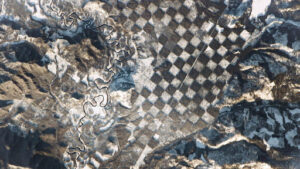
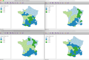
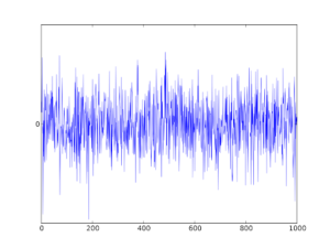
Figure 1. Typical spatial patterns.
(Left) A chessboard pattern illustrating strong negative spatial autocorrelation.
(Center) A clustered pattern showing positive spatial autocorrelation.
(Right) A spatial white-noise pattern with no detectable dependence.
Spatial Autocorrelation Signatures and Diagnostic Figures
Variogram
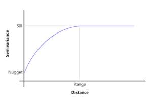
Figure 2. Empirical variogram.
The variogram summarizes how similarity between observations decreases with distance. The range indicates the scale of spatial dependence; the sill represents total variance; the nugget captures microscale variation or measurement error. Variograms are foundational tools for identifying process scale and spatial continuity.
Correlogram
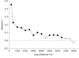
Figure 3. Spatial correlogram.
Correlograms plot spatial autocorrelation (e.g., Moran’s I) as a function of distance lag. They are particularly useful for detecting monotonic decay, oscillation, or long-range dependence, and for diagnosing isotropy versus anisotropy.
Periodogram
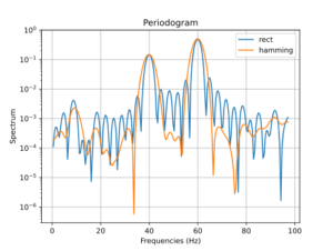
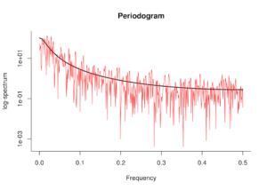
Figure 4. Spatial periodogram.
The periodogram decomposes spatial variation into frequency components, revealing dominant spatial wavelengths. Periodicity in the frequency domain can indicate repeating structures or regular spacing generated by underlying processes.
Wavelets

Figure 5. Wavelet-based spatial analysis.
Wavelets capture localized spatial structure across multiple scales. Unlike global methods, wavelets reveal where specific spatial scales dominate, making them well-suited for heterogeneous landscapes and nonstationary processes.
Process Example: Microevolutionary processes
- Isolation by Distance (IBD)
Produces smooth, monotonic decay of similarity with distance, visible in variograms and correlograms. - Migration
Introduces directional dependence (anisotropy), detectable as asymmetric autocorrelation structures. - Selection
Environmental gradients generate strong spatial structure even when stochastic variation is present.
In each case, inference of process depends on measuring spatial autocorrelation first.
Measure Before You Model
The core message here is simple: before fitting any spatial or space-time model, quantify the spatial autocorrelation in your data.
- If spatial dependence is present, spatial or space-time models are required.
- If spatial dependence is absent, aspatial models are both sufficient and preferable.
Spatial autocorrelation is not a statistical inconvenience—it is empirical evidence of process. Measuring it is the first step toward understanding how space-time processes shape the past, present, and future.
Get Started In Vesta
If this sounds daunting, it doesn’t have to be. Vesta is designed to make spatial autocorrelation analysis accessible to both beginners and experts. Not sure how to estimate a variogram or incorporate spatial structure into your model? Vesta includes automated variogram estimation and geostatistical interpolation that handles the technical details while keeping you in control of the analysis. See how it works in the tutorial below!
References
Jacquez, G. M. (1989). Implications of spatial autocorrelation in genetic and lake chemistry data. (PhD dissertation). State University of New York at Stony Brook.
Tobler, W. R. (1970). A computer movie simulating urban growth in the Detroit region. Economic Geography, 46(Supplement), 234–240.
Minkowski, Hermann. “Space and Time.” In The Principle of Relativity, by H. A. Lorentz, A. Einstein, and Hermann Minkowski, translated by W. Perrett and G. B. Jeffery, 73–91. Leipzig: B. G. Teubner, 1909. Lecture delivered September 21, 1908.
Sokal, R. R., & Wartenberg, D. E. (1983). A test of spatial autocorrelation analysis using an isolation-by-distance model. Genetics, 105(1), 219–237.
Sokal, R. R., & Wartenberg, D. E. (1983). Spatial autocorrelation analysis of biological populations. Biological Journal of the Linnean Society, 20(1), 53–69.