Local Cluster Analysis (Local Moran's I)

The Local Clustering method—also known as a Local Indicator of Spatial Autocorrelation (LISA)—identifies where statistically significant spatial clusters or outliers occur in your study area. It evaluates each location in relation to its neighbors to detect high-value clusters, low-value clusters, and spatial outliers. This method is essential for understanding the fine-scale geographic structure of disease risk, environmental exposure, or socio-demographic patterns.

The univariate Local Moran statistic is currently implemented in Vesta. This method tests for spatial autocorrelation in a single variable for each time period.

Test Statistics

The local Moran's I statistic compares the value recorded at location u₀ (kernel value) with values at J(u_0,). neighborhood locations u_j. This statistic is computed as:

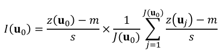
where m and s are the mean and standard deviation of the set of z-data. This local statistic is simply the product of the kernel value and the average of neighboring values; it can detect both positive and negative autocorrelations. It exceeds zero if the kernel and neighborhood averaged values jointly exceed the global mean m (High–High, HH cluster) or are jointly below m (Low–Low, LL cluster). LISA values are negative if the kernel and neighborhood mean values are on opposite sides of the global mean m, which indicates .

To test whether any test statistic, I(u₀), is significantly greater or smaller than 0 (i.e., presence of positive or negative spatial autocorrelation), one needs to know its probability distribution under the null hypothesis of spatial independence. The common way to generate such a reference distribution is to shuffle the set of z-values randomly and then to use the shuffled values to compute the neighborhood average while the kernel value remains the same (conditional randomization). In other words, the LISA statistic is computed for randomly distributed values in adjacent locations. This operation is repeated K times (K = 100 is the default value in Vesta) to compute the P-value of the test.

Impact of Missing Values in Local Cluster Analyses

If you have a dataset with missing values, calculations of the Local Moran statistics will be based on only those neighboring locations with data. Because the statistics are evaluated for significance with Monte Carlo randomizations (i.e., the differences in the distribution of observed statistic values can influence whether a particular value is judged as "rare"), removing one or more locations from a geography (thus creating missing values) can change results for all locations. You might observe this if you decide that a value or two represent outliers in your data, and re-run an analysis using missing values instead of the recorded ones. You will find that results for locations close to the one where missing values now occur change, but results for other locations may change as well due to the change in the overall distribution of the statistic.

Local Cluster Analysis Process

1. Click on the "Analyze" button from the side bar menu
2. Select "Exploratory Spatial Analysis", then click on "Local Cluster Analysis"
3. Select the dataset of interest
4. Select the variable of interest from the dataset drop-down menu.
5. Adjacency method is automatically selected based on the variable type
   • Nearest Neighbors uses the closest neighboring points or polygon centroids; The number of nearest neighbors can be modified to either expand or reduce the size of the neighborhood. Default is set to 16.
   • Polygon Adjacency uses the polygons that share a border or a corner (i.e., vertex) with the kernel polygon (1st order queen adjacency).
6. The number of randomizations is set to 100 by default; it can be increased for greater accuracy or decreased for faster calculations.
7. Select "Run" to execute the method
   • Look at the bottom of the workspace for a message indicating that the task is in process or has been completed.
8. Results are displayed in a new workspace, and are also saved in the right-hand Data panel.

Local Cluster Analysis Summary and Results

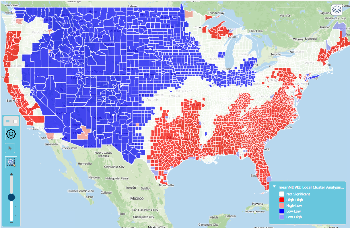
The Local Moran test results provide insight into the local spatial autocorrelation, and offer insight into data clusters (similar values) and outliers (value different from neighbors). Four quantities are calculated: z-score, Local Moran's I for each location, p-value, and Local Moran Class. Each observation/location is classified into one of the following four categories:

1. HH - the location is part of a significant high-high correlation cluster, meaning that the location has high autocorrelated and surrounded by other high autocorrelated neighbors.
2. LL - the location is part of a significant low-low correlation cluster, meaning that the location has low autocorrelation and surrounded by other low autocorrelation neighbors.
3. HL - the location is an outlier with high autocorrelation but surrounded by neighbors with low autocorrelation.
4. LH - the location is an outlier with low autocorrelation but surrounded by neighbors with high autocorrelation.

If the data is labelled with NS, the Local Moran's I is not significantly different from zero (p-value greater than 0.05).

Each of the four new variables are automatically mapped in the result workspace.

Global Moran's I is a measure of spatial autocorrelation ranging from -1 to +1:

• Positive values (0 to +1): Similar values tend to cluster together geographically. High values are near other high values, and low values are near other low values.
• Negative values (-1 to 0): Dissimilar values tend to be near each other. High values are surrounded by low values, and vice versa.
• Values near 0: No spatial autocorrelation; values are randomly distributed across space. The closer the value is to +1 or -1, the stronger the spatial pattern.

Summary Report (displayed in workspace)

A summary report is given with classification of clusters in the data analyzed. See the content at the top of the summary report for data-specific interpretation and results.

The Moran Scatterplot (displayed in workspace)

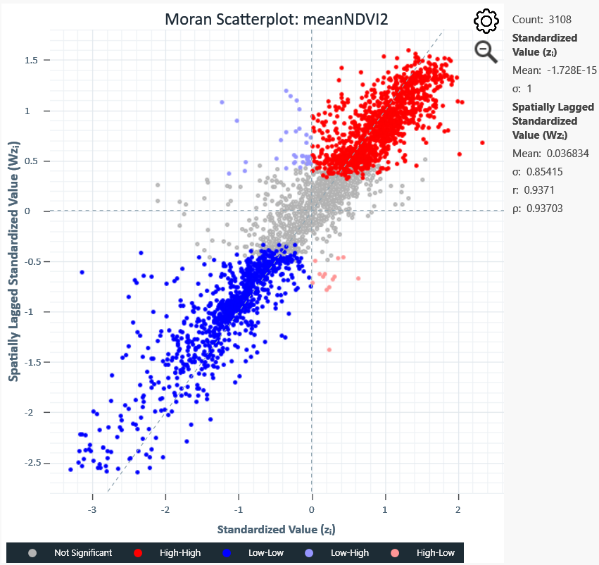
This chart plots each location's standardized value (x-axis) against the average of its neighbors (y-axis).

• Upper-right quadrant (High-High) and lower-left quadrant (Low-Low): Confirm clustering trends.
• Upper-left quadrant (Low-High): Low-value locations surrounded by high-value neighbors.
• Lower-right quadrant (High-Low): High-value locations surrounded by low-value neighbors.
• Grey points: Statistically not significant localities, neither clusters nor outliers.

Histogram of Cluster Results (displayed in workspace)

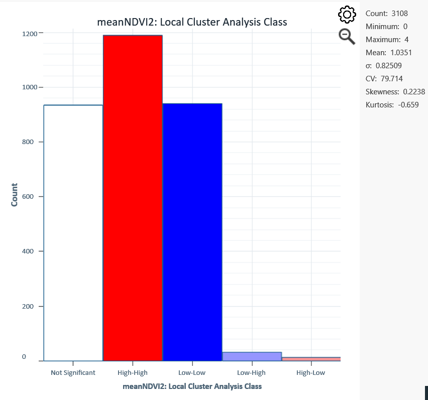
The histogram shows counts of objects classified as Not Significant, Low-Low, Low-High, High-High, and High-Low. The histogram is interactive; click or brush-select any bar to see the count and location of those localities.