Geostatistical Interpolation

One of the strengths of geostatistical interpolation is its ability to incorporate multiple data layers in the prediction. In other words, it capitalizes on the correlation between observations and among variables to make predictions at any unsampled location. It is particularly useful when the variable of interest, called a primary variable, is supplemented by secondary data that were collected in greater numbers and over different sets of locations. Note that all variables need to share a common subset of sampling locations in order to assess their cross-correlation.

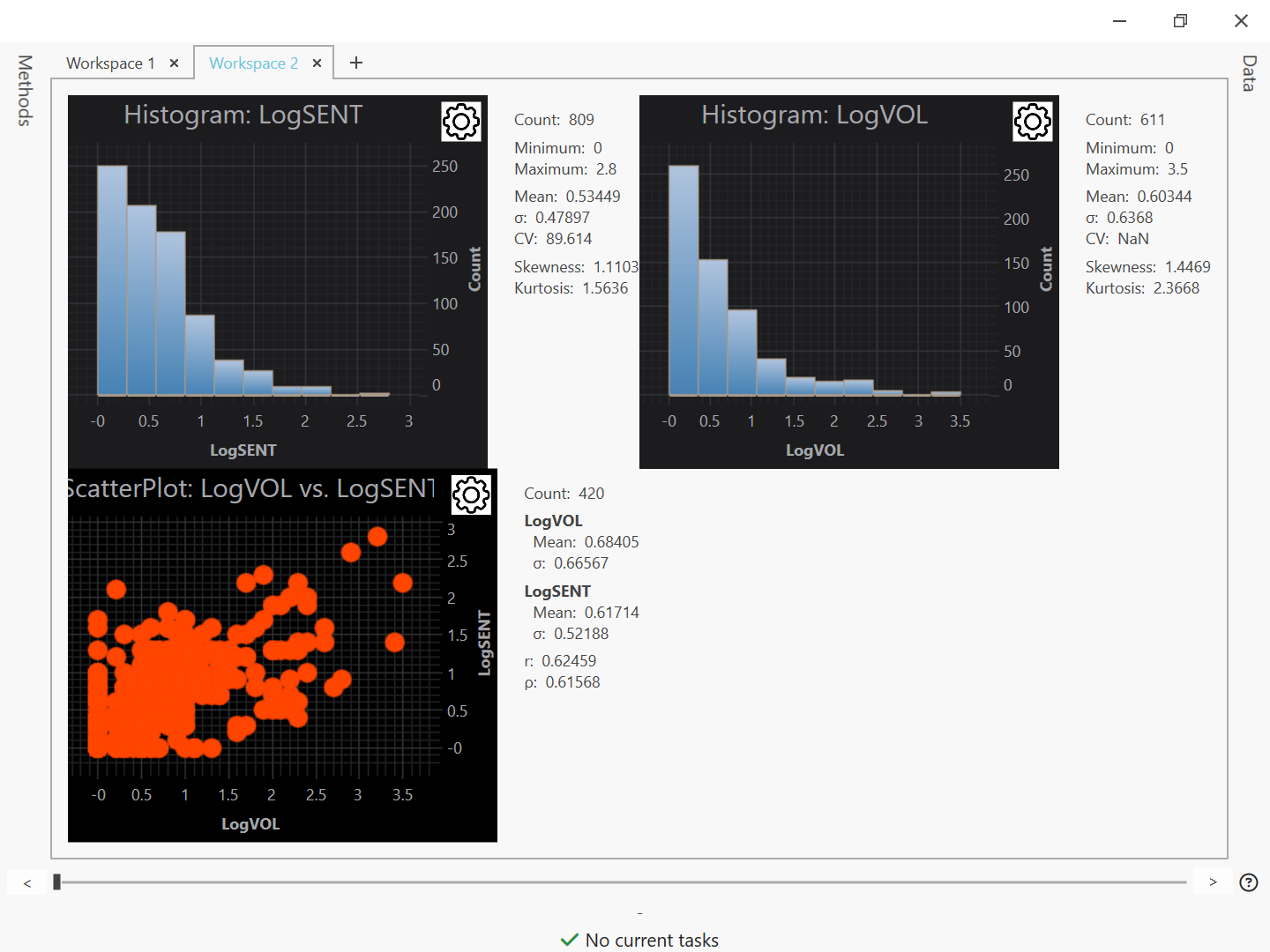
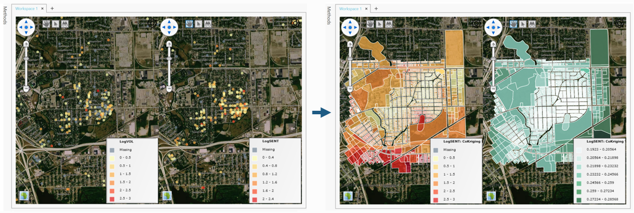
In the example below, water lead level was measured at two different sets of locations during two separate sampling campaigns: 1) 809 sentinel sites, and 2) 611 voluntary sites, where 420 samples share the same location.

Data collected at sentinel sites are considered more reliable and cokriging is used to incorporate the voluntary data as secondary source of information in predicting water lead concentrations (left map) and the associated cokriging variance (right map) at all residential tax parcels in the City of Flint.

Choosing the Variable to Interpolate

Kriging fills in the gaps between measurements. It only makes sense for a quantity that genuinely varies smoothly over space — a pollutant concentration, a soil property, a rainfall depth. A variable whose value is an administrative fact rather than a field measurement has nothing for the variogram to find.

The variable's type decides the kind of kriging performed, and this is derived automatically rather than chosen: a continuous variable is kriged directly; a categorical variable is kriged as indicators, giving one estimated probability per category plus a most-likely-category map; a compositional group is kriged in log-ratio space and back-transformed, so the estimated parts still sum to the whole.

Note that interpolation assumes the sample locations are not themselves informative about the value. If sites were placed because the value was expected to be high — around a known source, for example — the estimate inherits that bias, and the variance map will not warn you about it.

Ordinary kriging also assumes a constant mean across the study area. A strong regional trend is better removed first, in Variography with covariates, than left for the kriging system to absorb.

Kriging Types

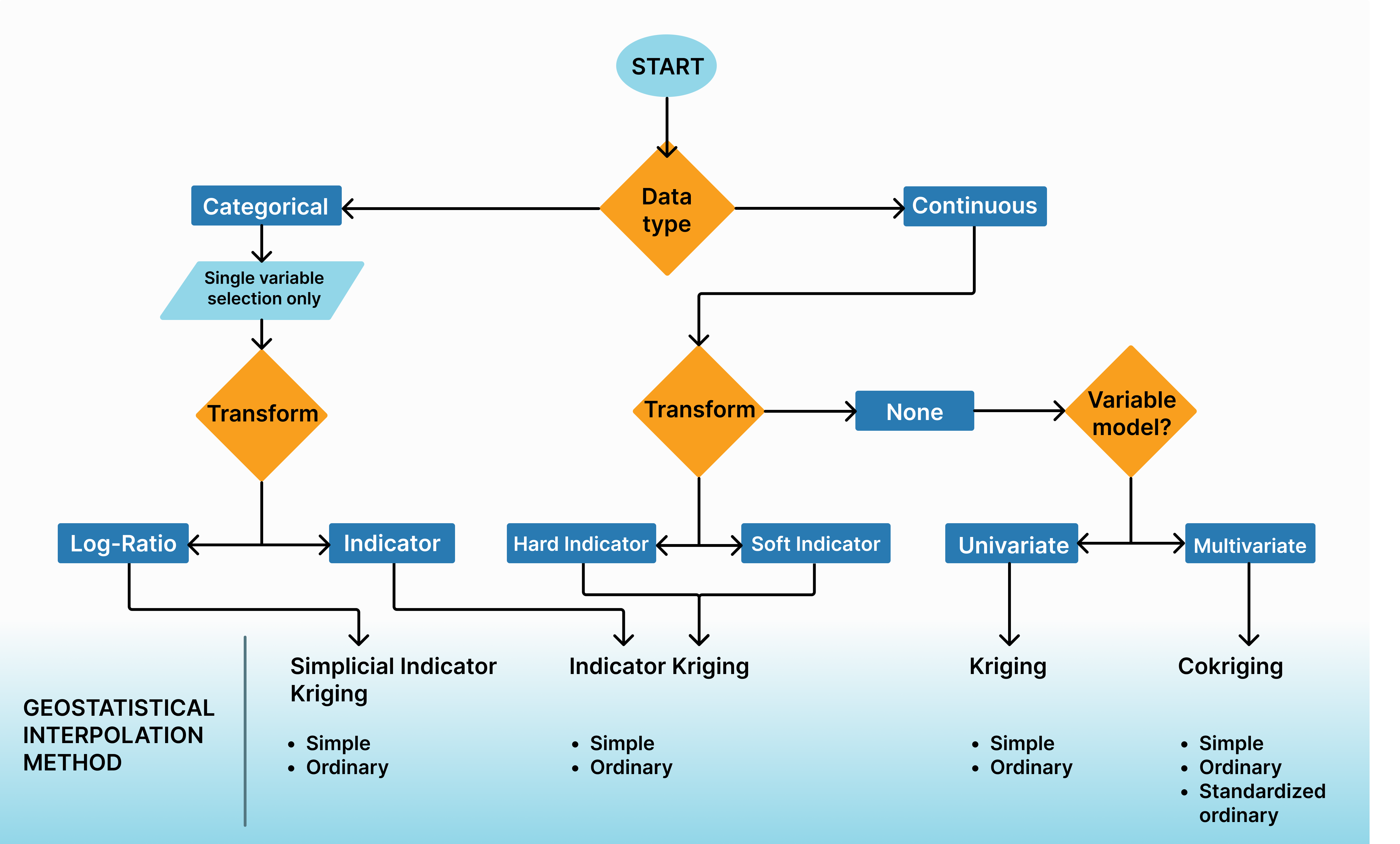
Vesta allows the calculation of a wide variety of kriging estimators depending on the type of variable (e.g., continuous vs categorical), the number of variables (1 to 3), and the type of data transform (i.e., no transform, indicator transform, logratio transform). See flowchart below.

Anisotropic Kriging

When the variogram model used for interpolation has anisotropy fitted (see Anisotropy and Directional Variograms), kriging automatically honors the directional structure it describes — predictions draw more heavily on nearby observations along the fitted direction of stronger correlation. No additional configuration is needed in the kriging dialog itself; the anisotropy carries through from the variogram model selected in Process Steps, step 5. This also applies to cokriging (multi-variable fits using a linear model of coregionalization).

Categorical Variables

Categorical variables are a way to "tag" data as being of a particular category, such as the material used to construct a water pipe (lead, copper, PVC), soil type (silt, clay, sand), or land uses (agrarian, industrial, residential). Many times data is collected in several places across a larger area to get enough information to interpolate remaining spots based on the category of the surroundings. However, categorical variables cannot be interpolated “as is”.

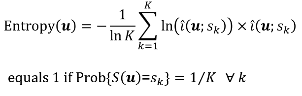
Instead, the probability of occurrence of each category s_k is predicted, then the category s_k' with the largest probability is selected as the most probable and used as prediction: S ̂_ML (u)=s_k' if i ̂(u;s_k' )=Prob{S(u)=s_k'}> i ̂(u;s_k ) ∀ k ≠k'. Uncertainty about the prediction can be captured using any measure of the spread of the probability distribution. For example, the relative local entropy ranges between 0 and 1 (maximum uncertainty if all estimated probabilities are the same):

Indicator Kriging with Categorical Variables

This interpolation requires the coding of all observations S(u_α ) into indicators of presence/absence of each of the K categories, followed by the application of indicator kriging to each set of indicators:

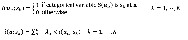
Where the kriging weights λ_α are solutions of a system of linear equations.

Simplicial Indicator Kriging with Categorical Variables

A limitation of indicator kriging is that since the probabilities for all categories are estimated individually, there is no guarantee that at each location u the K estimated probabilities i ̂(u;s_k ) sum up to 1. Such constraint can be satisfied by treating the categorical variable as compositional (Aitchinson, 1986 ).

In that case, the data are first transformed into log-ratios, which are then interpolated by kriging, followed by their back-transform to obtain estimated probabilities => {i ̂(u_α;s_k ), k=1,⋯,K} that will by construction sum to 1 and be valued between 0 and 1.

The three steps, which are accomplished automatically in Vesta , are thus:

1. Transform each categorical data S(u_α ) into a set of log-ratios:
2. Kriging of log-ratios at unsampled location u:
3. Transform estimated logratios back into probabilities:

Validation of Interpolation with Categorical Variables

For categorical variables, Vesta offers the option of assessing the accuracy of the prediction using a second dataset that was not used in the prediction stage. The two datasets available are thus:

1. Estimated probabilities and most likely category predicted at a set of N test locations
2. Observed category and corresponding indicators at these N same locations:

These data are used by Vesta to calculate:

• Contingency Table: S ̂_ML (u_β ) vs S(u_β ), which highlights the number of locations that are correctly classified (diagonal elements of the table) as well as the number of locations that are assigned to the incorrect category.

• ROC curve and AUC (Area Under the Curve) statistic for each category s_k: The ROC curve plots the probability of false alarm (false positive) versus the probability of detection (vertical axis); see example below (Swets, 1988 ; Goovaerts, 2017)

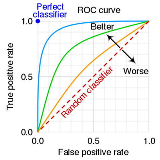
The accuracy of the prediction is quantified using the relative area under the ROC curve (AUC statistic), which ranges from 0 (worst case) to 1 (best case). The AUC is equivalent to the probability that the classifier will rank a randomly chosen positive instance (e.g., presence of a lead service line) higher than a randomly chosen negative instance (e.g., absence of lead service line).

Continuous Variables with no Transform

This is the most common situations where the goal is to predict the value of one continuous variable using observations for that variable (kriging estimator) and other related variables that are sampled more densely (cokriging). The algorithms implemented in Vesta are described here <<<<>>>>>> and in Goovaerts (1997).

Continuous Variables with Indicator Transform

Two common features of environmental datasets are the occurrence of a few very large concentrations (hot-spots) and the presence of data below the detection limit (censored observations). Extreme values can strongly affect the characterization of spatial patterns, (i.e., estimation of the variogram) and subsequently the prediction. Several approaches exist to handle strongly positively skewed histograms (Saito and Goovaerts, 2000 ).

One way to attenuate the impact of extreme values is to use more robust statistics and estimators. The non-parametric approach of indicator kriging (IK) falls within that category (Journel, 1983 ). The basic idea is to discretize the range of variation of the environmental attribute by a set of thresholds z_k (e.g. deciles of sample histogram, detection limit, regulatory threshold) and to transform each observation into a vector of indicators of non-exceedence of each threshold:

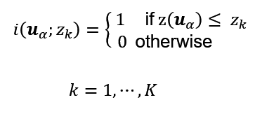
Where z(u_α) is the observation of variable Z at location u_α.

The user specifies the number K of thresholds that are then calculated as equiprobable percentiles of the sample frequency distribution, F(.), as: z_k=F-1(p_k) with {p_k= p_min+(k-1)×((1-p_min ))/K,k=1,⋯,K}. For example, K=9 would result in the calculation of 9 thresholds as the 9 deciles of the dataset. Kriging is then applied to the set of indicators and estimated values are assembled to form a conditional cumulative distribution function (ccdf). The mean and the variance of the probability distribution can be used as an estimate of the attribute value and the uncertainty attached to the prediction (Goovaerts, 2009).

In several situations, observations themselves can be uncertain or imprecise; e.g., measurement errors for laboratory data, or small number problem for health outcome. In that case, one might not know with certainty whether the attribute value z(u) exceeds a particular threshold z_k or not. Like in the previous case, the user specifies the number K of thresholds that are then calculated as equiprobable percentiles of the sample frequency distribution, F(.). The indicators are called “soft” because they are valued between 0 and 1, instead of being binary 0/1 as for hard indicators (no uncertainty).

Soft indicators are cumulative frequencies and can be calculated for three types of distributions in Vesta, as shown in the variography section on soft indicators.

Post-processing Indicator Kriging Estimates

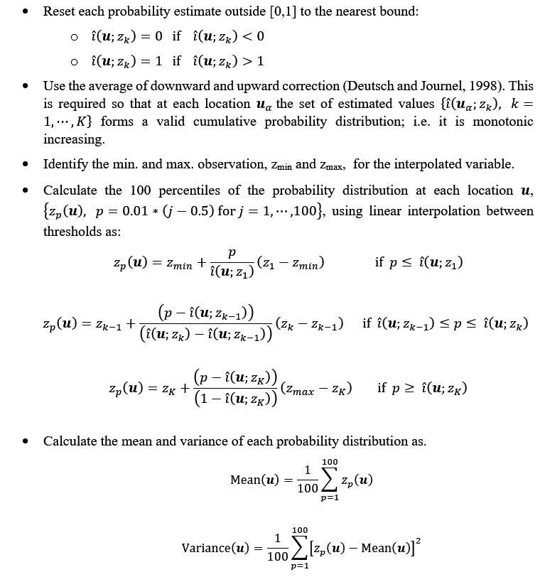
Like for categorical variables, since the probabilities for all thresholds are estimated individually, there is no guarantee that at each unsampled location u the K estimated probabilities i ̂(u;z_k ) form a “valid” cumulative probability distribution function; that is 0≤i ̂(u;z_k )≤1 ∀ k and i ̂(u;z_k' )≤i ̂(u;z_k ) if z_(k^' ) ≤ z_k. In addition, the set of K probabilities need to be interpolated within each class (zk,zk+1] and extrapolated beyond the smallest and the largest thresholds to build a continuous model for the probability distribution.

Following the procedure described in Goovaerts (1997) the set of K probabilities {i ̂(u;z_k ), k=1,⋯,K} underwent the following correction:

Kriging Estimators

Material forthcoming.

Please see variogram estimators in the interim.

Process Steps

The GeoStatistical analysis can be invoked from Vesta's AI Advisor by stating in plain english the desired analysis type and selecting from the options presented by the Advisor.

The following process steps can also be used if the user chooses to step through manually, using the Guided Analyze wizard (see Analysis Introduction):

1. Click on the "Analyze" button from the side bar menu, or search for "Geostatistical Interpolation" from the Guided Analyze wizard's Analysis step.
2. Choose Automatic, Guided, or Full control guidance.
3. Variable — choose the variable or compositional group to interpolate (see Choosing the Variable to Interpolate, above). The dataset follows the variable; there is no separate source-dataset picker.
4. Variogram — choose where the variogram comes from:
   • Fit automatically — Vesta fits a model for this variable at run time. This is the only option available under Automatic guidance.
   • Saved variogram — reuse a model already fitted for this variable, so that repeated runs are comparable. Only models fitted for the selected variable are offered, since a variogram belongs to the variable it was fitted on.
   • Fit one here — insert the Experimental, Model, and Anisotropy steps used by the Variography method, useful when the automatic fit looks wrong, the nugget is doing too much work, or the continuity is suspected to have a direction. The fitted variogram can optionally be kept and saved to the project.
5. Prediction surface — choose where the estimates go, and how kriging is run:
   • Existing geography fills in the gaps of the dataset the measurements came from; New grid builds a regular grid over the data's extent by specifying a cell size, without needing to create a separate destination geography first. Grid cell size is mainly a cost decision: halving it quadruples the work, and a cell finer than the spacing between measurements adds resolution without adding information.
   • Kriging type: Ordinary (the usual choice — the local mean is estimated from each neighborhood) or Simple (use only when the mean is known and constant; estimates are pulled toward that mean where data is sparse). Standardized ordinary kriging is also available for cokriging.
   • Neighbours per estimate — too few makes the surface noisy; too many pulls every estimate toward the global mean, a slower way of drawing a flat map.
6. Validation — optionally cross-validate the fit (see Cross-Validation, below). For categorical variables specifically, see Validation of Interpolation with Categorical Variables, above, for the contingency table and ROC/AUC statistics available there.
7. Run — review the choices made in the previous steps, including the discretization count (the number of random points used to discretize any object in the input and output geographies, 10 by default), then run. Nothing is written to the project until the run completes.
8. Summary — results are shown under a "kriging folder" located in the Output Geography, in the Data panel to the right.

Cross-Validation

Kriging always produces a surface, and the surface always looks plausible — cross-validation is what tells you whether it's any good. It holds measurements back, predicts them from the rest, and reports how far off the predictions were. This costs a second pass over the data, but it is the only honest check of the fit.

Five methods are available:

• None — skip cross-validation.
• Leave one out — the most thorough method: every measurement is predicted from all the others. Also the slowest, since it solves one kriging system per observation.
• K-fold — the same idea in batches; a sensible default on a large dataset.
• Train/test split — the cheapest method, and the noisiest, since the result depends on which measurements happen to land in the held-out part.
• Separate dataset — the strongest evidence of all, since the held-out measurements were never available to the model at any point. Requires a second dataset measuring the same quantity at different locations.

Cross-validation error statistics are written to a separate Cross-Validation Results workspace, not to the interpolation summary. Read them alongside the kriging variance map, not instead of it: the variance map says where the surface is uncertain from the sample geometry, while the cross-validation errors say whether that uncertainty was honest.

Kriging Output

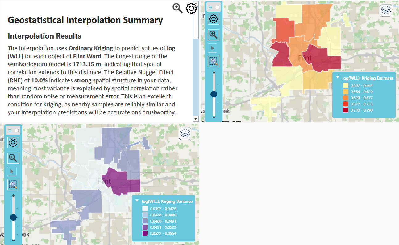
After running geostatistical interpolation (kriging), the workspace typically shows several key elements: a summary of the interpolation analysis, a map of the predicted values (kriging estimate), and a map of the prediction uncertainty or error (kriging variance). These visualizations help you understand both the spatial pattern of the interpolated variable and the confidence in those predictions.

The summary report contains substantial information on the specific results of an interpolation. Expand each summary section to learn more about your results.