Regression in Vesta

Regression methods are a set of tools for assessing variation in one variable (the dependent variable) at set levels of another variable or variables (the explanatory, or independent, variables). Unlike measures of correlation, like those that also accompany the scatter plots in Vesta, these tools assume that there is a functional dependence of values of the dependent variable on the level of the independent variable(s).

Vesta fits a single Regression model that automatically takes the form appropriate to your dependent variable: an ordinary least squares (OLS) model for a continuous (Double or Integer) dependent variable, or a logistic model for a binary (yes/no) dependent variable, which estimates a probability rather than a level. This is an aspatial method — the geographic coordinates of the observations are not used in the fit itself. If you think the relationship between your variables varies across your study area rather than holding uniformly, see Geographically Weighted Regression instead.

Aspatial Linear (OLS) Regression

In traditional linear regression, a statistical model is fit to a set of N observations such that a dependent variable y can be expressed in terms of one or more independent variables, and a residual, or error, term. Assumptions of linear regression models include:

1. Independent observations
2. Normally distributed variables, and
3. Homoscedasticity, or similar variances in the dependent variable across different values or levels of the independent variable(s)

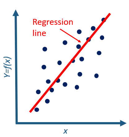
The figure below shows a dataset of N =23 points, plotted so that y, the variable we would like to be able to predict, is shown on the vertical axis, and a single independent variable (x) is shown on the horizontal axis. The goal of the linear regression modeling exercise is to find the linear function that provides the best prediction of y; that is, it produces the smallest errors, measured as the squared difference between the observed value of y, and the value of y from the regression line at the same value of x.

Note that the term "linear" refers to the linear combination of parameters in the model, and that the graph that results from a linear regression model does not have to be a straight line.

Regression Equation

In the linear regression model, the independent variable observations are regarded as fixed, and all other variables (y, and the error term) are considered random. One way of expressing a linear regression model with an unspecified number of independent variables is shown below. The x part of the β_jx_ij component drops out when j =0, leading to the y-intercept, β₀.

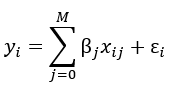
• i = 1 .... N (number of observations)
• j = 0 ... M (number of independent variables)
• y_i = dependent variable
• β_j = regression coefficients
• x_ij = the j'th variable at observation i
• ε_i = residual variable

Logistic Regression

When the dependent variable is binary, Vesta automatically switches the fit to a logistic model, estimating the probability of the outcome rather than a continuous level. The choice is determined entirely by the dependent variable's type — there is no separate "Logistic Regression" method to select; the badge shown while choosing variables says which form you are about to run.

Choosing Variables

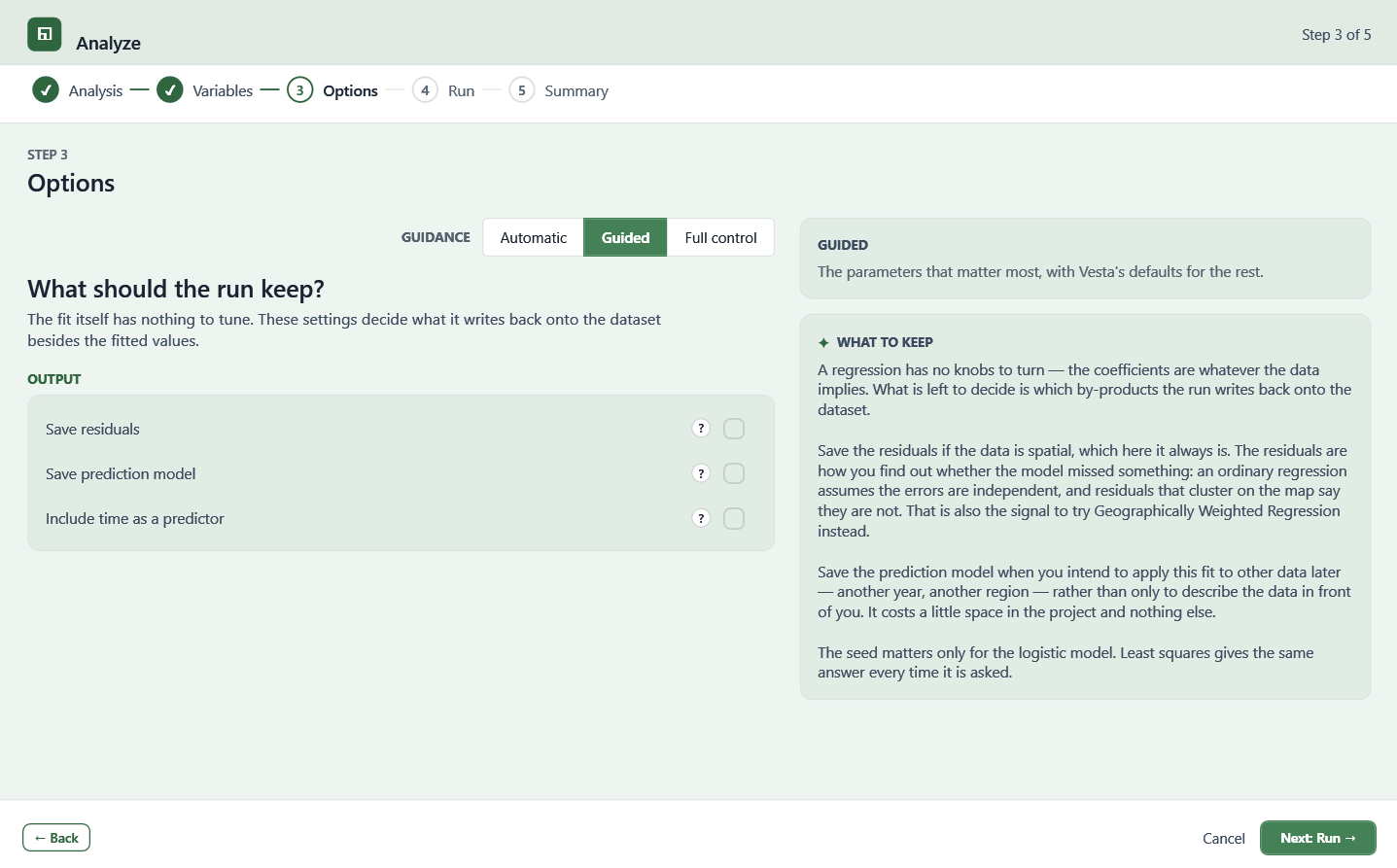
A regression explains one variable — the dependent variable — as a function of the others. The fit runs on the dependent variable's own dataset, and only variables on that same layer can serve as explanatory variables.

Explanatory variables should be things you believe act on the response, not everything the dataset happens to hold — two predictors that measure nearly the same thing make the coefficients unstable and their signs unreliable, even when the overall fit looks good. Under Automatic guidance, Vesta derives the predictor list for you and leaves out variables that were written by earlier analyses, since regressing on another method's output produces a fit that explains everything and means nothing.

Options

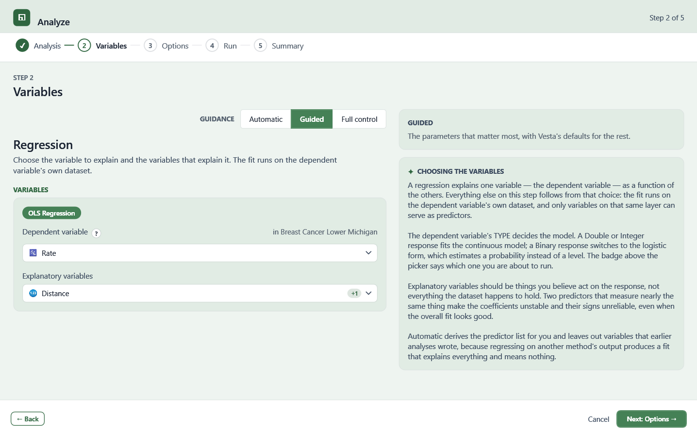
A regression fit itself has no parameters to tune — the coefficients are whatever the data implies. What can be configured is which by-products the run writes back onto the dataset:

• Save residuals — recommended when the data is spatial, which it always is in Vesta. The residuals are how you find out whether the model missed something: ordinary regression assumes the errors are independent, and residuals that cluster on the map say they are not — the signal to try Geographically Weighted Regression instead.
• Save prediction model — save the fit so it can be applied to other data later, such as another year or another region, rather than only describing the data in front of you.
• Include time as a predictor.

The random seed used to fit the model matters only for the logistic form; the least-squares fit used for a continuous outcome gives the same answer every time it is run.

Process Steps

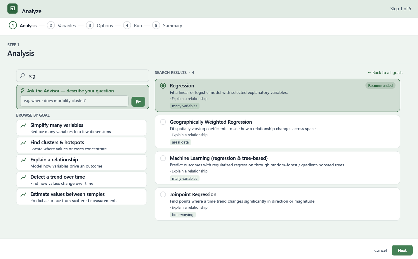
1. Click on the "Analyze" button from the side bar menu, or search for "Regression" from the Guided Analyze wizard's Analysis step.

   

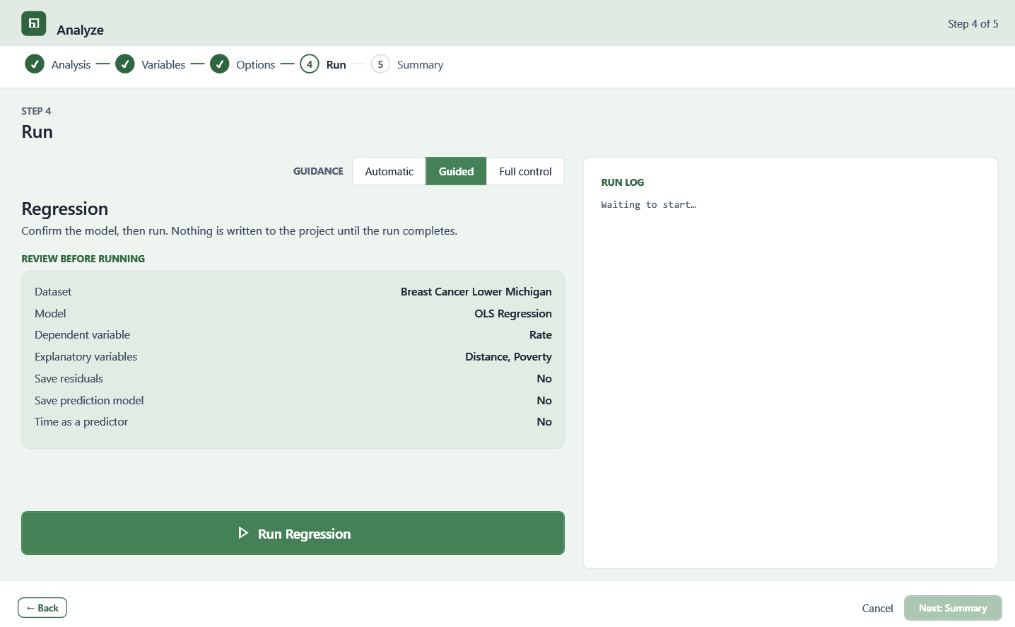
2. Choose Automatic, Guided, or Full control guidance. See Analysis Introduction for more on the Guided Analyze wizard.

3. Choose the dependent variable to explain and the explanatory variables that explain it (see Choosing Variables, above).
4. Choose what the run should keep (see Options, above).

5. Review the model summary and select "Run Regression."

   

6. Results are saved in the Data panel to the right.

Regression Output

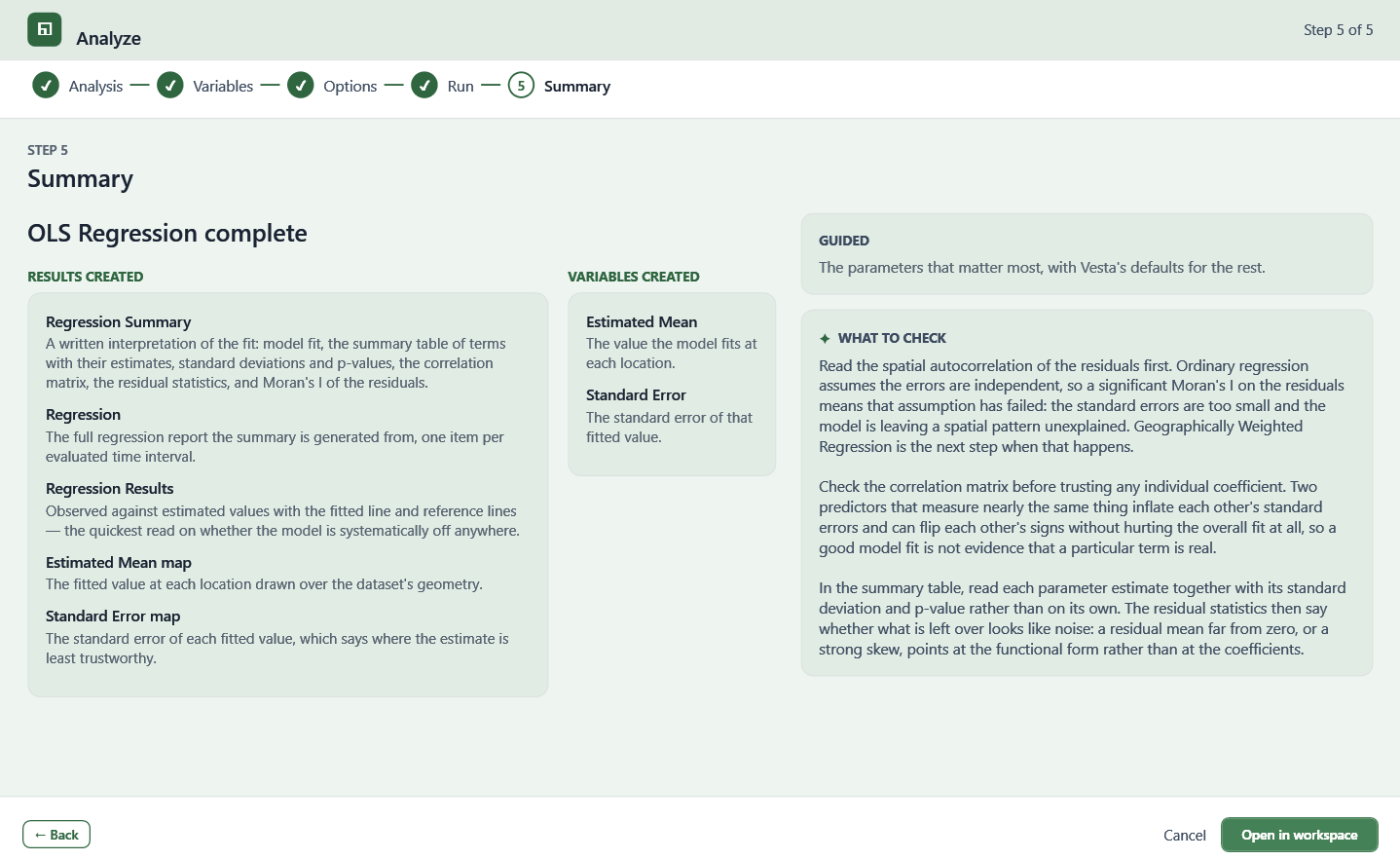
Running a regression produces:

• Regression Summary — a written interpretation of the fit: model fit, a summary table of terms with their estimates, standard deviations, and p-values, the correlation matrix, residual statistics, and Moran's I of the residuals.
• Regression — the full report the summary is generated from, one item per evaluated time interval.
• Regression Results — a plot of observed against estimated values with the fitted line and reference lines, the quickest read on whether the model is systematically off anywhere.
• Estimated Mean map — the fitted value at each location.
• Standard Error map — the standard error of each fitted value, showing where the estimate is least trustworthy.

Note that for datasets with both spatial and temporal components, the regression model is fitted for each time interval, and results are reported for each.

What to Check

• Read the spatial autocorrelation of the residuals first. Ordinary regression assumes the errors are independent, so a significant Moran's I on the residuals means that assumption has failed — the standard errors are too small, and the model is leaving a spatial pattern unexplained. Geographically Weighted Regression is the next step when that happens.
• Check the correlation matrix before trusting any individual coefficient. Two predictors that measure nearly the same thing inflate each other's standard errors and can flip each other's signs without hurting the overall fit at all — a good model fit is not evidence that a particular term is real.
• Read each parameter estimate together with its standard deviation and p-value, not on its own. The residual statistics then say whether what is left over looks like noise: a residual mean far from zero, or a strong skew, points at the functional form rather than at the coefficients.