Importing Data into Vesta

Now it is time to get your data file into Vesta! Data is added from the Add Data hub in the main rail (see Navigating Vesta), which offers two paths: pulling from an online source, or bringing in a file of your own. For troubleshooting, see the Troubleshooting page in the section above.

Adding Data from an Online Source

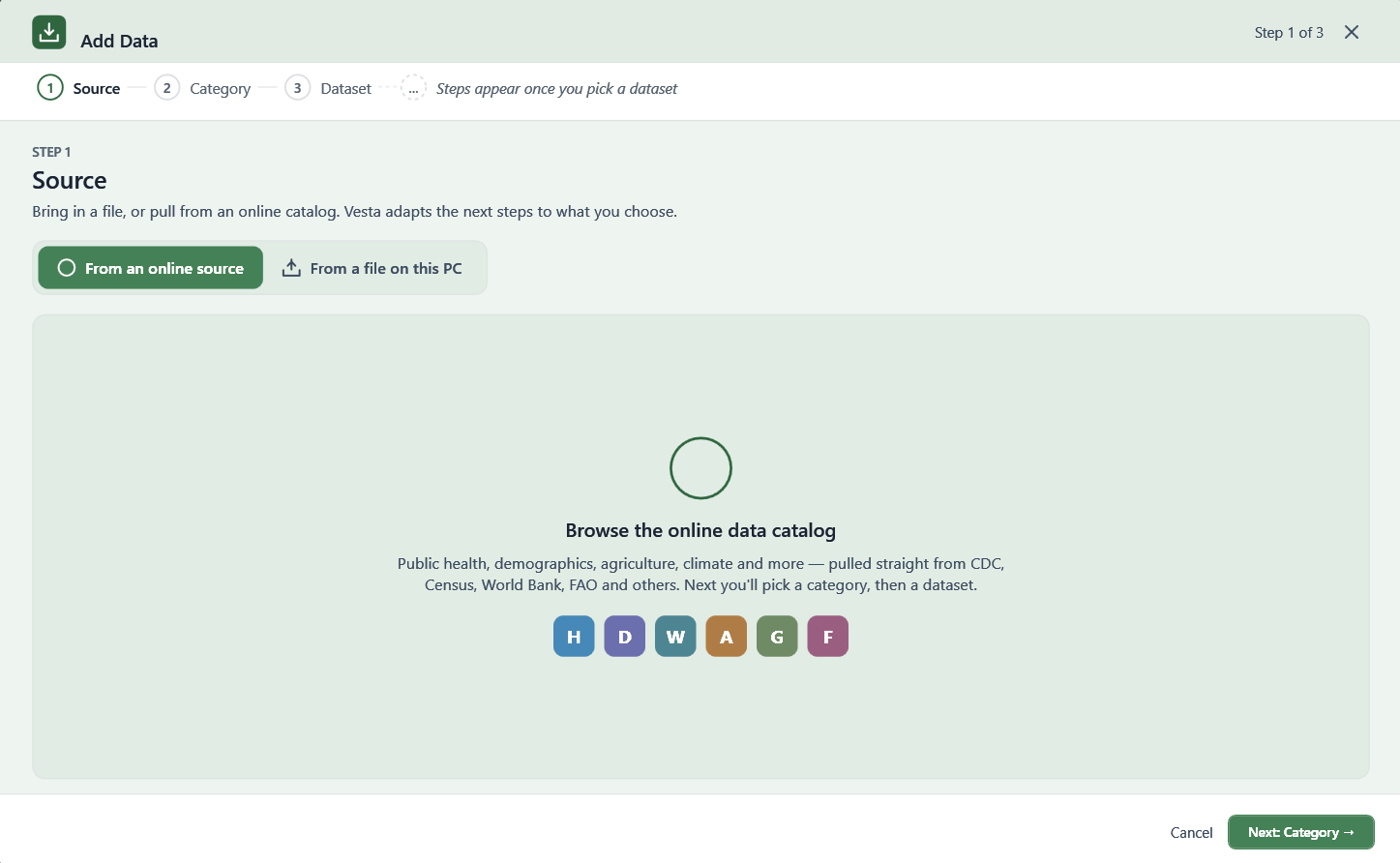
Step 1: Source

Choose From an online source.

Step 2: Category

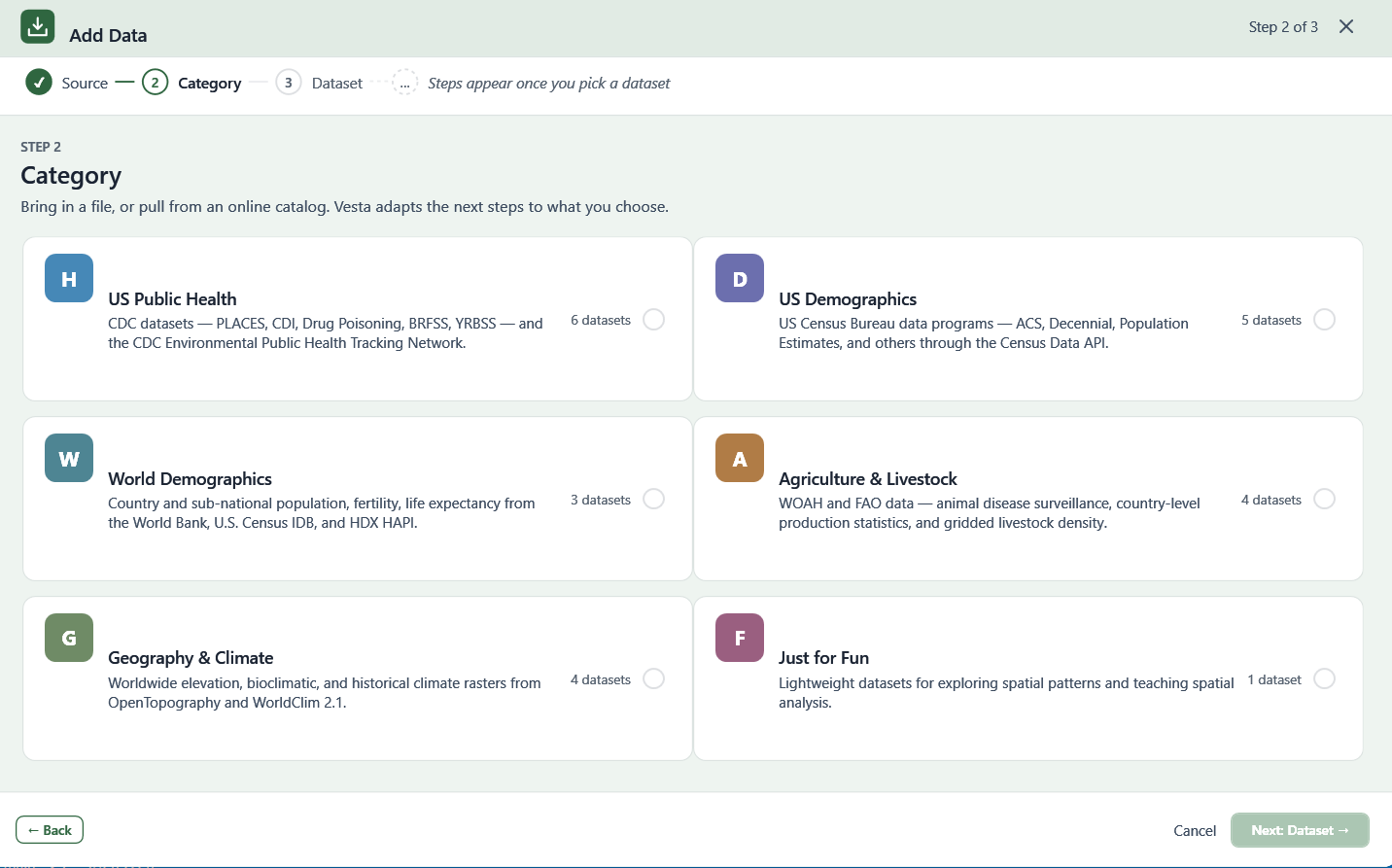
Pick a category:

• US Public Health — CDC datasets including PLACES, Chronic Disease Indicators (CDI), Drug Poisoning, BRFSS, YRBSS, and the CDC Environmental Public Health Tracking Network.
• US Demographics — U.S. Census Bureau data programs, including ACS, Decennial, and Population Estimates, through the Census Data API.
• World Demographics — country and sub-national population, fertility, and life expectancy data from the World Bank, U.S. Census IDB, HDX HAPI, and WorldPop.
• Agriculture & Livestock — WOAH and FAO data, including animal disease surveillance, country-level production statistics, and gridded livestock density and production systems.
• Geography & Climate — worldwide elevation, bioclimatic, and historical climate rasters from OpenTopography and WorldClim, plus MODIS satellite imagery and GRIP4 road density.
• Just for Fun — lightweight datasets for exploring spatial patterns and teaching spatial analysis.

See Online Data Sources for the full catalog of datasets available within each category.

Step 3: Dataset

Select a specific dataset from the list — each entry shows its coverage (geographic levels, year range, number of indicators) and a "Dataset info" link with more detail. Search the list by name if you know what you're looking for.

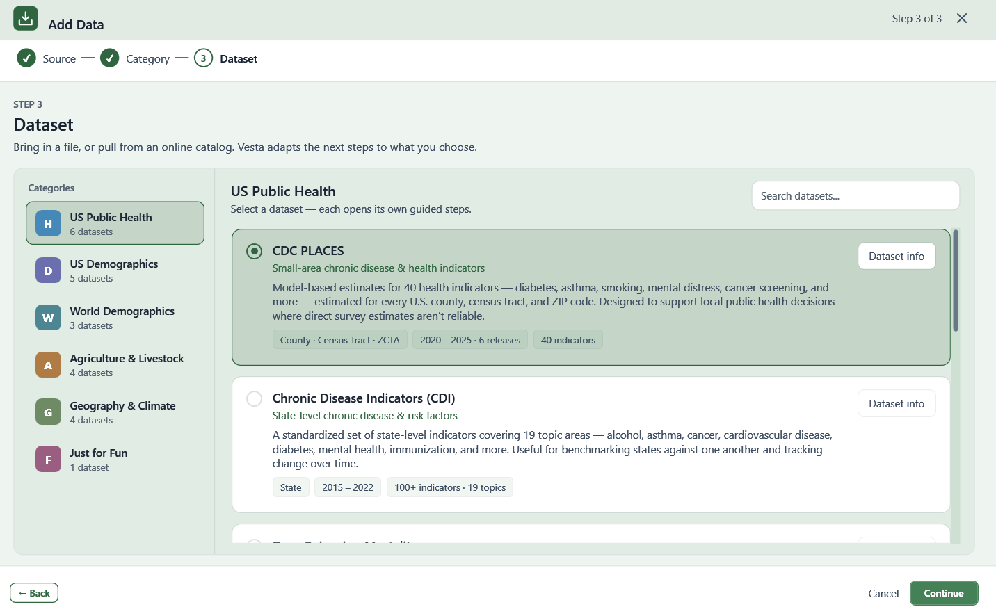
The steps that follow depend on which dataset you picked. As an example, importing from CDC PLACES continues with:

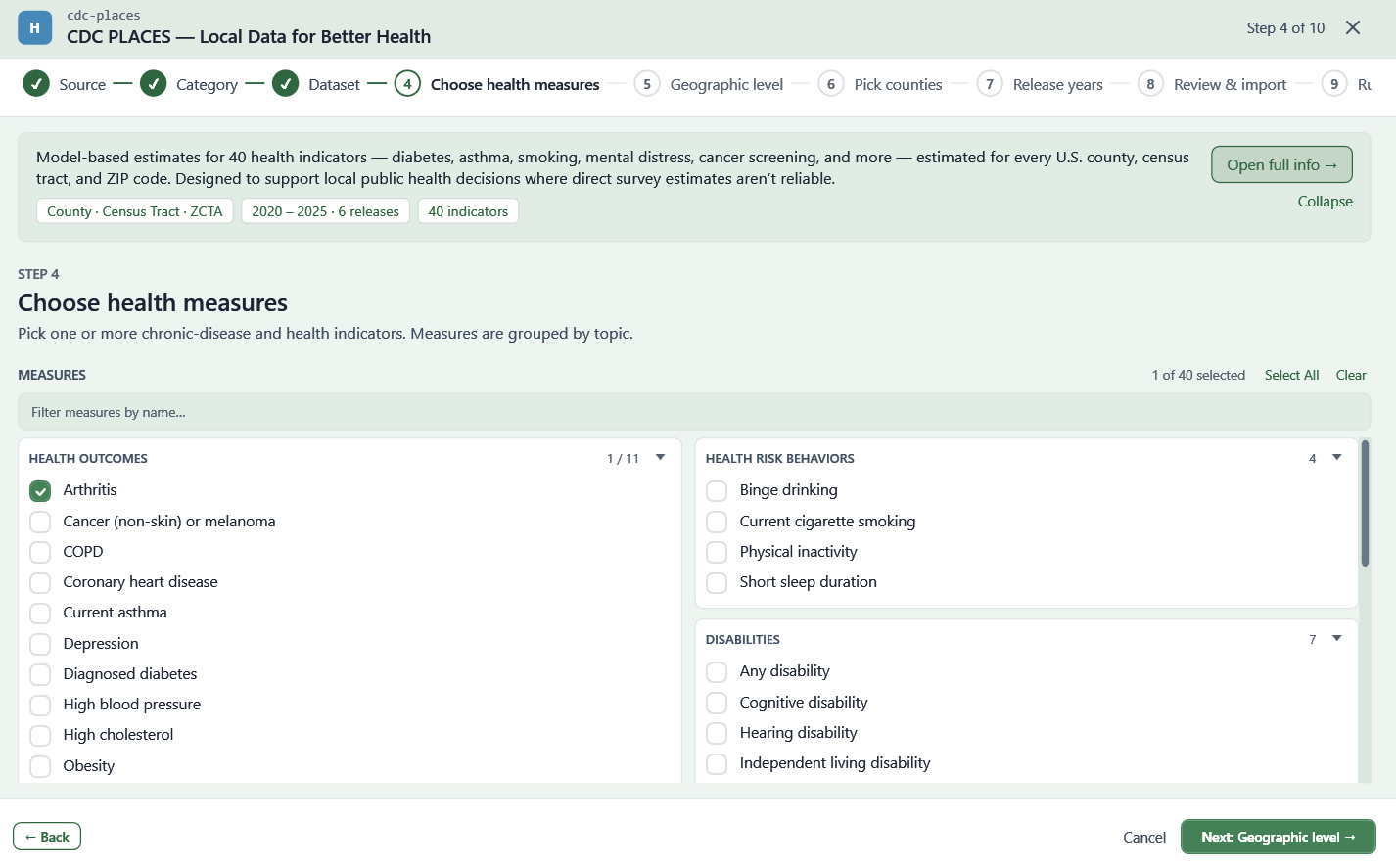
Step 4: Choose Health Measures

Pick one or more indicators, grouped by topic (Health Outcomes, Health Risk Behaviors, Disabilities, and more).

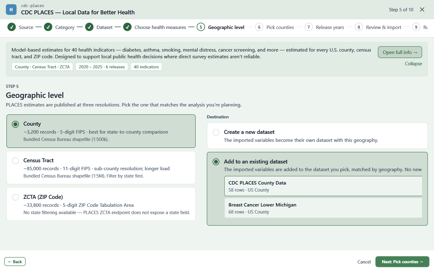
Step 5: Geographic Level and Destination

Choose the resolution that fits your analysis (e.g., County, Census Tract, or ZCTA), each with its own record count and tradeoffs. Alongside this, choose a Destination: create a new dataset with this geography, or add the imported variables to an existing dataset in your project, matched by geography.

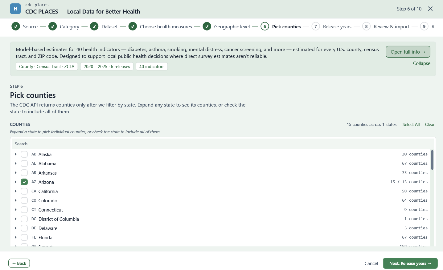
Step 6: Pick Counties

A searchable, expandable state/county tree for narrowing which areas to include.

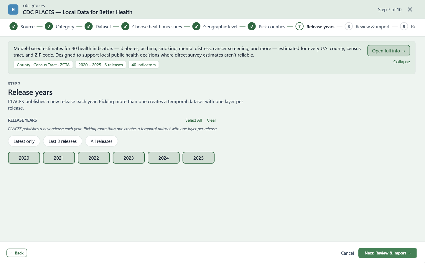
Step 7: Release Years

Pick one or more available releases; picking more than one creates a time-varying dataset with one layer per release.

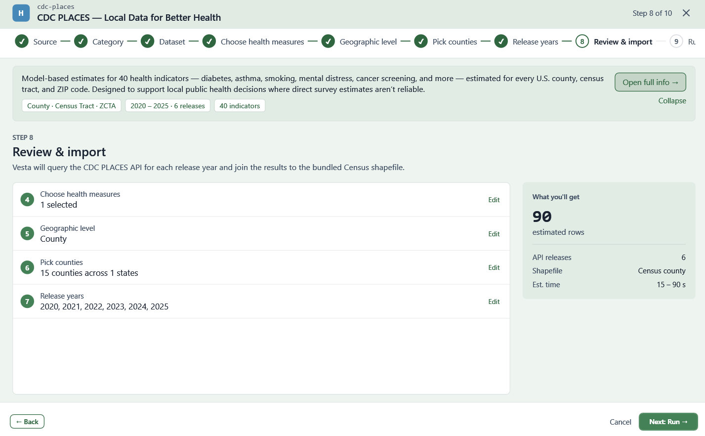
Step 8: Review & Import

A recap of your choices alongside an estimate of what you'll get (row count, number of releases, estimated time).

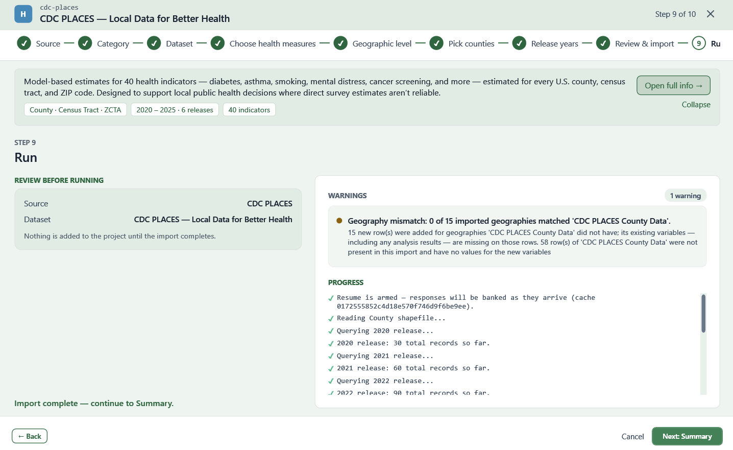
Step 9: Run

The import runs, and any issues are reported directly — for example, if some of the geographies you imported didn't match an existing dataset you're adding to, Vesta reports how many rows were added, and which existing rows were left without values for the new variables.

Resuming an Interrupted Import

If an online import is cancelled or fails partway through, Vesta keeps what it already downloaded. Returning to the same import shows a Resume available panel instead of starting over, with the choice to Continue from where it stopped, Adjust selection and continue, Start over, or Discard the banked progress.

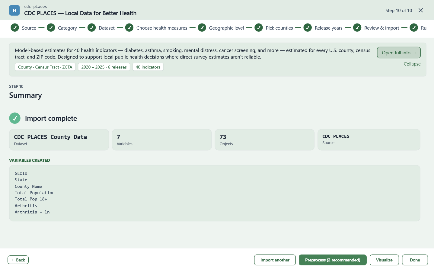
Step 10: Summary

Shows the resulting dataset, its variables, and a log of what happened, with options to import another dataset, preprocess, visualize, or finish.

Other online sources follow the same overall Category → Dataset → source-specific pattern, with their own set of questions in between (for example, an area of interest instead of counties, or a variable list instead of health measures).

Adding Data from a Local File

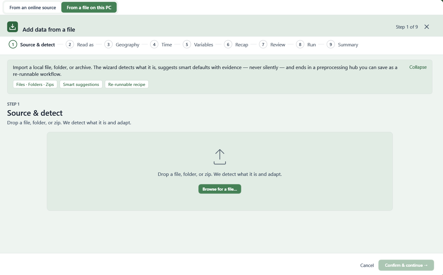
Choose From a file on this PC in Step 1 to bring in your own file, folder, or zip archive — Vesta detects what it is and adapts the remaining steps.

Step 1: Source & Detect

Drop or browse for a file, folder, or archive.

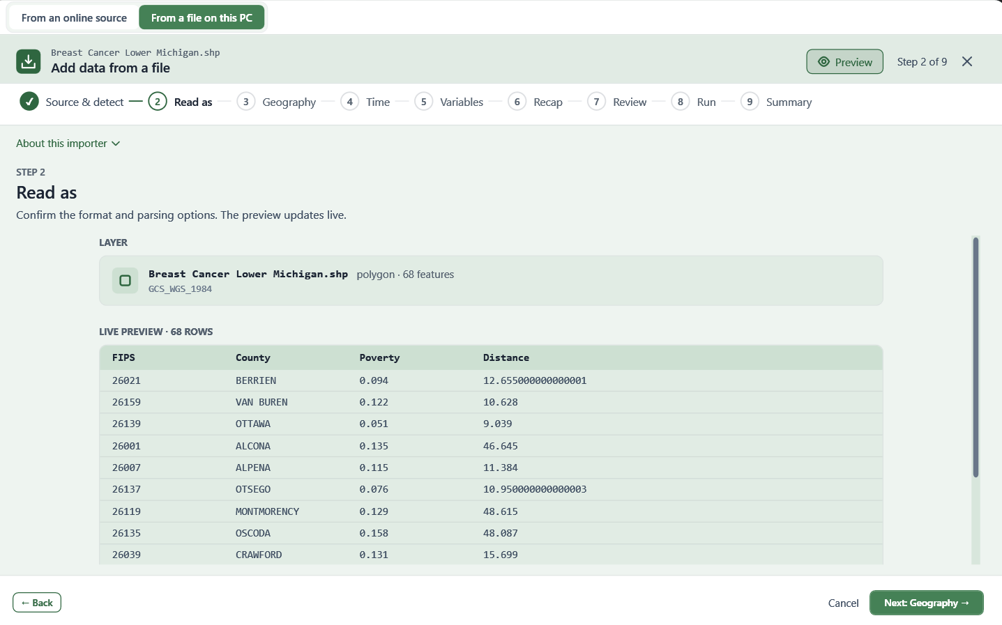
Step 2: Read As

Confirm the detected format and parsing options, with a live preview of the data. Vesta detects whether a file is a table, vector features, or a raster grid, and adapts the available options accordingly — for a delimited text file, this includes the delimiter, text encoding, and whether the first row is a header. For CSV, TXT, and Excel files, Vesta also finds the true header and data rows on its own when a published table wraps title rows or trailing footnotes around the real table, and reports which rows it skipped.

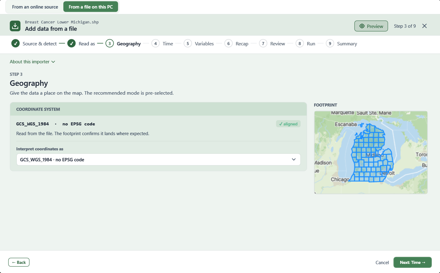
Step 3: Geography

Choose how to place the data:

• Join to geography — match a key column in the file against an existing dataset already in your project, with a live match-quality preview (for example, "1,428 / 1,428 matched — good match"). Joining to one of Vesta's built-in standard geographies (such as Census tracts or counties) contributes only that geography's boundary — your file's own columns come through under their own names, without picking up the boundary's own attribute fields.
• Own geometry — use the geometry carried by the file itself. Vesta reads its coordinate system and lets you override this if needed, including specifying a custom EPSG code or reading it from a .prj file. A footprint preview confirms the data lands where expected on the map.
• Build from coordinates — create geometry from X/Y or latitude/longitude columns in the file.

Step 4: Time

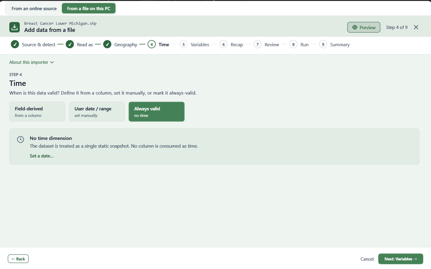
Choose how the data varies over time: derived from a column, a date or range you set manually, or always valid (no time dimension). When deriving time from a column, choose whether each row represents a single Observation (a single time per row) or a Range (a start and an end), pick the time column, and set the granularity (e.g., Yearly) — Vesta shows the date range it detected in the data.

Step 5: Variables

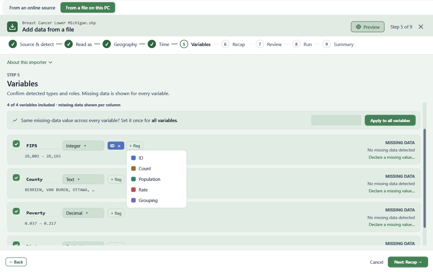
Confirm the detected type of each variable, assign a role (ID, Count, Population, Rate, or Grouping), and declare a missing-data value per column, or apply one value to every column at once — applied consistently no matter how the data is being placed on the map. Select All / Clear controls make working through a long variable list faster.

The type shown for each variable is a real choice, not just a preview: picking Categorical here imports the column with its category labels directly, without a separate preprocessing step afterward. Vesta also recognizes identifier-style codes — a ZIP code, FIPS code, or GEOID with leading zeros or too many digits to be a whole number — and reads them as text so their leading zeros and full digit count are preserved, with a dismissible banner naming any columns read this way (you can still override the type yourself). Automatically suggested flags like ID are shown here too, and whatever you set on this step — including clearing a flag Vesta suggested — is exactly what carries through to the imported dataset.

Step 6: Recap

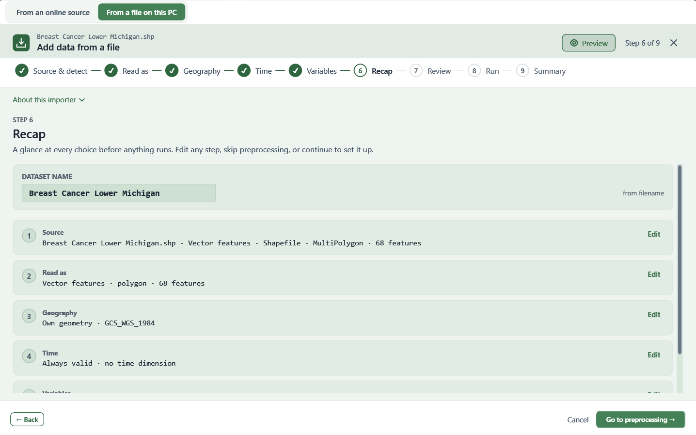
Review and, if needed, edit any earlier step, including the dataset's name.

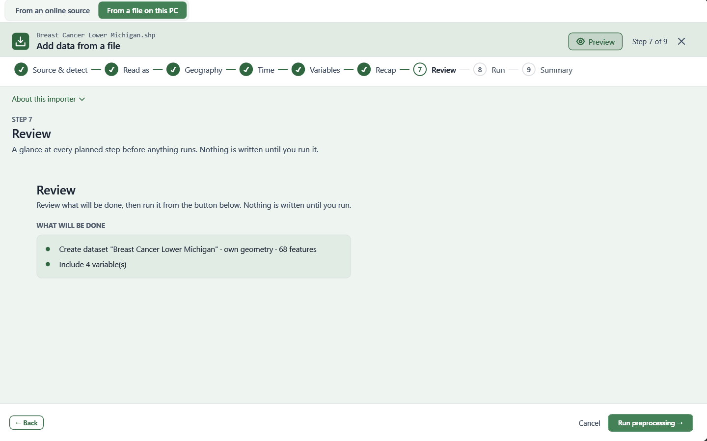
Step 7: Review

A final summary of what will be created before anything is written.

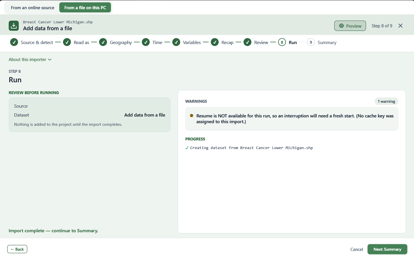
Step 8: Run

The import runs, with progress and any warnings shown as it goes.

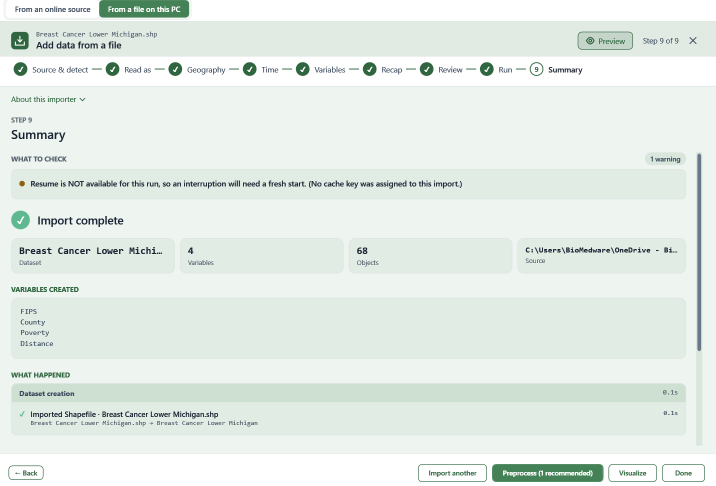
Step 9: Summary

Shows the resulting dataset, its variables, and a log of what happened.

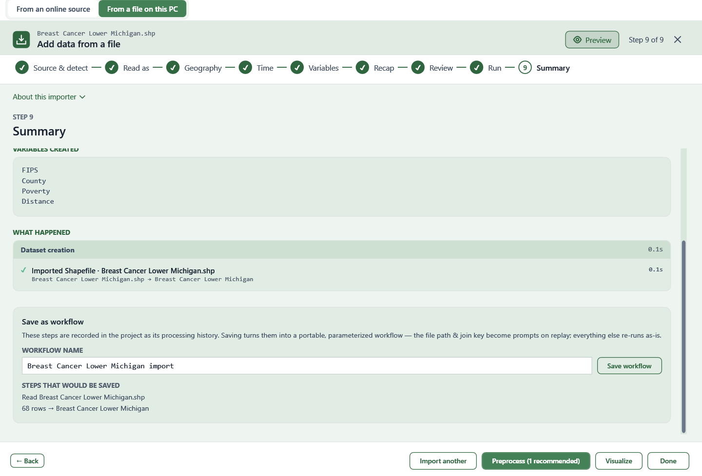
From here, you can save the import as a reusable workflow (see Workflows) — the file path and any join key become prompts when you replay it, and everything else runs the same way again. From the Summary screen, you can also continue directly into Preprocess, Visualize, or finish.

Notes on Missing Data and Identifiers

Whether importing online or from a file, a variable can be flagged as the dataset's ID so it can be matched against an existing dataset later. If an existing dataset's identifier variable isn't available to match against, it first needs to be designated as an ID variable from the Data panel: right-click the variable's name and select "Modify". See Other Data Modifications for more information.

Notes on Moving Point Data

Some point data changes location over time — a GPS track, an animal's movements, or a person's residential history. Vesta can hold this as moving-point geometry: instead of collapsing a person or object to a single location, every recorded fix is kept, with a position stored for each object at each point in time. Distance and speed between fixes are calculated geodesically, directly from latitude and longitude, rather than from the map's projected coordinates. Once imported, a moving-point dataset can be drawn as a trail on a map — see Creating a Map.